grids.mixins.mathops.DenseMathOpsMixin.dense_covariant_gradient#

Compute the covariant gradient of a dense-representation tensor field on a grid.

For a tensor field \(T_{\ldots}^{\ldots}({\bf x})\), the covariant gradient is the rank \(rank(T)+1\) tensor \(T_{\ldots\mu}^{\ldots}({\bf x})\) such that

\[T_{\ldots \mu}^{\ldots}({\bf x}) = \partial_\mu T_{\ldots}^{\ldots}({\bf x}).\]

Parameters:

tensor_field (array-like) – The tensor field on which to compute the partial derivatives. This should be an array-like object with a compliant shape (see Notes below).
field_axes (list of str) – The coordinate axes over which the tensor_field spans. This should be a sequence of strings referring to the various coordinates of the underlying coordinate_system of the grid. For each element in field_axes, tensor_field’s i-th index should match the shape of the grid for that coordinate. (See Notes for more details).
out (array-like, optional) – An optional buffer in which to store the result. This can be used to reduce memory usage when performing computations. The shape of out must be compliant with broadcasting rules (see Notes). out may be a buffer or any other array-like object.
output_axes (list of str, optional) –
The axes of the coordinate system over which the result should span. By default, output_axes is the same as field_axes and the output field matches the span of the input field.

This argument may be specified to expand the number of axes onto which the output field is computed. output_axes must be a superset of the field_axes.
in_chunks (bool, optional) – Whether to perform the computation in chunks. This can help reduce memory usage during the operation but will increase runtime due to increased computational load. If input buffers are all fully-loaded into memory, chunked performance will only marginally improve; however, if buffers are lazy loaded, then chunked operations will significantly improve efficiency. Defaults to False.
edge_order ({1, 2}, optional) – Order of the finite difference scheme to use when computing derivatives. See numpy.gradient() for more details on this argument. Defaults to 2.
pbar (bool, optional) – Whether to display a progress bar when in_chunks=True.
pbar_kwargs (dict, optional) – Additional keyword arguments passed to the progress bar utility. These can be any valid arguments to tqdm.tqdm().
**kwargs – Additional keyword arguments passed to dense_compute_gradient_covariant().

Returns:

The computed partial derivatives. The resulting array will have a field shape matching the grid’s shape over the output_axes and an element shape matching that of field but with an additional (ndim,) sized dimension containing each of the partial derivatives for each index.

Return type:

array-like

Notes

Broadcasting and Array Shapes:

The input tensor_field must have a very precise shape to be valid for this operation. If the underlying grid (including ghost zones) has shape grid_shape = (G_1,...,G_ndim), then the spatial dimensions of the field must match exactly grid_shape[axes]. Any remaining dimensions of the field are treated as densely populated tensor indices and therefore must each have ndim elements.

Thus, if a (G1,G3,ndim,ndim,...) field is passed with field_axes = ['x','z'] (in cartesian coordinates), then the resulting output array will have shape (G1,G3,ndim,ndim,...,ndim) and out[...,1] == 0 because the field does not contain any variability over the y variable.

If output_axes is specified, then that resulting grid will be broadcast to any additional grid axes necessary.

When out is specified, it must match (exactly) the expected output buffer shape or an error will arise.

Chunking Semantics:

When in_chunks=True, chunking is enabled for this operation. In that case, the out buffer is filled iteratively by performing computations on each chunk of the grid over the specified output_axes. When the computation is performed, each chunk is extracted with an additional 1-cell halo to ensure that numpy.gradient() attains its maximal accuracy on each chunk.

Note

Chunking is (generally) only useful when out and tensor_field are array-like lazy-loaded buffers like HDF5 datasets. In those cases, the maximum memory load is only that required to load each individual chunk. If the out buffer is not specified, it is allocated fully anyways, making chunking somewhat redundant.

See also

dense_element_wise_partial_derivatives: Generic form for general array-valued fields.
dense_contravariant_gradient: Contravariant gradient of a tensor field.
dense_compute_gradient_covariant: Low-level callable version.

Examples

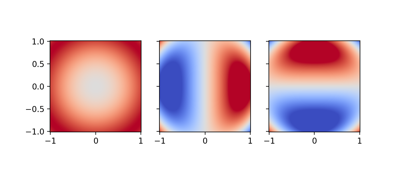
Covariant Gradient of a Scalar Field

The easiest example is the derivative of a generic scalar field.

>>> from pymetric.grids.core import UniformGrid
>>> from pymetric.coordinates import CartesianCoordinateSystem2D
>>> import matplotlib.pyplot as plt
>>>
>>> # Create the coordinate system
>>> cs = CartesianCoordinateSystem2D()
>>>
>>> # Create the grid
>>> grid = UniformGrid(cs,[[-1,-1],[1,1]],[500,500],chunk_size=[50,50],ghost_zones=[[2,2],[2,2]],center='cell')
>>>
>>> # Create the field
>>> X,Y = grid.compute_domain_mesh(origin='global')
>>> Z = np.sin((X**2+Y**2))
>>>
>>> # Compute the partial derivatives.
>>> derivatives = grid.dense_covariant_gradient(Z,['x','y'])
>>>
>>> fig,axes = plt.subplots(1,3,sharey=True,sharex=True,figsize=(7,3))
>>> _ = axes[0].imshow(Z.T,origin='lower',extent=grid.gbbox.T.ravel(),vmin=-1,vmax=1,cmap='coolwarm')
>>> _ = axes[1].imshow(derivatives[...,0].T,origin='lower',extent=grid.gbbox.T.ravel(),vmin=-1,vmax=1,cmap='coolwarm')
>>> _ = axes[2].imshow(derivatives[...,1].T,origin='lower',extent=grid.gbbox.T.ravel(),vmin=-1,vmax=1,cmap='coolwarm')
>>> plt.show()

(Source code, png, hires.png, pdf)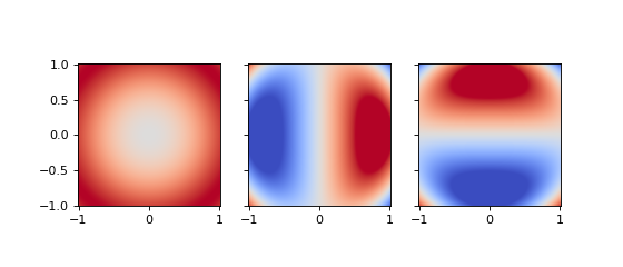

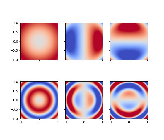
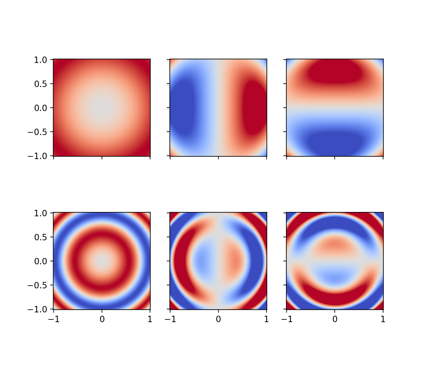
../_images/grids-mixins-mathops-DenseMathOpsMixin-dense_covariant_gradient-1.png

Derivatives of a vector field:

Similarly, this can be applied to vector field (or more general tensor field).

>>> from pymetric.grids.core import UniformGrid
>>> from pymetric.coordinates import CartesianCoordinateSystem2D
>>> import matplotlib.pyplot as plt
>>>
>>> # Create the coordinate system
>>> cs = CartesianCoordinateSystem2D()
>>>
>>> # Create the grid
>>> grid = UniformGrid(cs,[[-1,-1],[1,1]],[500,500],chunk_size=[50,50],ghost_zones=[[2,2],[2,2]],center='cell')
>>>
>>> # Create the field
>>> X,Y = grid.compute_domain_mesh(origin='global')
>>> Z = np.stack([np.sin((X**2+Y**2)),np.sin(5*(X**2+Y**2))],axis=-1) # (504,504,2)
>>>
>>> # Compute the partial derivatives.
>>> derivatives = grid.dense_covariant_gradient(Z,['x','y'])
>>>
>>> fig,axes = plt.subplots(2,3,sharey=True,sharex=True,figsize=(7,6))
>>> _ = axes[0,0].imshow(Z[...,0].T,origin='lower',extent=grid.gbbox.T.ravel(),vmin=-1,vmax=1,cmap='coolwarm')
>>> _ = axes[0,1].imshow(derivatives[...,0,0].T,origin='lower',extent=grid.gbbox.T.ravel(),vmin=-1,vmax=1,cmap='coolwarm')
>>> _ = axes[0,2].imshow(derivatives[...,0,1].T,origin='lower',extent=grid.gbbox.T.ravel(),vmin=-1,vmax=1,cmap='coolwarm')
>>> _ = axes[1,0].imshow(Z[...,1].T,origin='lower',extent=grid.gbbox.T.ravel(),vmin=-1,vmax=1,cmap='coolwarm')
>>> _ = axes[1,1].imshow(derivatives[...,1,0].T,origin='lower',extent=grid.gbbox.T.ravel(),vmin=-5,vmax=5,cmap='coolwarm')
>>> _ = axes[1,2].imshow(derivatives[...,1,1].T,origin='lower',extent=grid.gbbox.T.ravel(),vmin=-5,vmax=5,cmap='coolwarm')
>>> plt.show()

(Source code, png, hires.png, pdf)

../_images/grids-mixins-mathops-DenseMathOpsMixin-dense_covariant_gradient-2.png

Expanding to output axes:

In some cases, you might have a field \(T_{ijk\ldots}(x,y)\) and you may need \(\partial_\mu T_{ijk\ldots}(x,y,z)\). This can be achieved by declaring the output_axes argument.

>>> from pymetric.coordinates import CartesianCoordinateSystem3D
>>>
>>> # Create the coordinate system
>>> cs = CartesianCoordinateSystem3D()
>>>
>>> # Create the grid
>>> grid = UniformGrid(cs,[[-1,-1,-1],[1,1,1]],[50,50,50],chunk_size=[5,5,5],ghost_zones=[2,2,2],center='cell')
>>>
>>> # Create the field
>>> X,Y = grid.compute_domain_mesh(origin='global',axes=['x','y'])
>>> Z = np.stack([np.sin((X**2+Y**2)),np.sin(5*(X**2+Y**2)),np.zeros_like(X)],axis=-1) # (54,54,3)
>>>
>>> # Compute the partial derivatives.
>>> derivatives = grid.dense_covariant_gradient(Z,['x','y'],output_axes=['x','y','z'])
>>> derivatives.shape
(54, 54, 54, 3, 3)

Inconsistent Input Field:

Note that in the previous example, we required

Z = np.stack([np.sin((X**2+Y**2)),np.sin(5*(X**2+Y**2)),np.zeros_like(X)],axis=-1) # (54,54,3)

to have an additional element. This is because dense_covariant_gradient() requires dense representations. The same result can be achieved under less strict conventions with dense_element_wise_partial_derivatives().

Z = np.stack([np.sin((X**2+Y**2)),np.sin(5*(X**2+Y**2))],axis=-1) # (54,54,3)
derivatives = grid.dense_covariant_gradient(Z,['x','y'],output_axes=['x','y','z'])
ValueError: Incompatible full field shape.
  Expected: (54, 54, 3)
  Found   : (54, 54, 2)

grids.mixins.mathops.DenseMathOpsMixin.dense_covariant_gradient#

This Page