differential_geometry.dense_ops.dense_gradient#
- differential_geometry.dense_ops.dense_gradient(tensor_field: ndarray, rank: int, ndim: int, *varargs, basis: Literal['contravariant', 'covariant'] | None = 'covariant', inverse_metric_field: ndarray | None = None, out: ndarray | None = None, edge_order: Literal[1, 2] = 2, field_axes: Sequence[int] | None = None, output_indices: Sequence[int] | None = None, **kwargs) ndarray[source]#
Compute the gradient of a tensor field in the specified output basis.
This function computes the component-wise partial derivatives of a tensor field with respect to its grid coordinates, and optionally raises the resulting index using a provided inverse metric.
- Parameters:
tensor_field (
numpy.ndarray) –Tensor field of shape
(F_1, ..., F_m, N, ...), where the last rank axes are the tensor index dimensions. The partial derivatives are computed over the first m axes.Hint
Because this function is a low-level callable, it does not enforce the density of the elements in the trailing dimensions of the field. This can be used in some cases where the field is not technically a tensor field.
rank (
int) – Number of trailing axes that represent tensor indices (i.e., tensor rank). The rank determines the number of identified coordinate axes and therefore determines the shape of the returned array.ndim (
int) – The number of total dimensions in the relevant coordinate system. This determines the maximum allowed value formand the number of elements in the trailing dimension of the output.*varargs –
Grid spacing for each spatial axis. Follows the same format as
numpy.gradient(), and can be:A single scalar (applied to all spatial axes),
A list of scalars (one per axis),
A list of coordinate arrays (one per axis),
A mix of scalars and arrays (broadcast-compatible).
If field_axes is provided, varargs must match its length. If axes is not provided, then varargs should be
tensor_field.ndim - rankin length (or be a scalar).inverse_metric_field (
numpy.ndarray) –Inverse metric tensor with shape
(..., ndim, )or(..., ndim, ndim), where the leading dimensions (denoted here asF1, ..., F_n) must be broadcast-compatible with the grid (spatial) portion of tensor_field.Specifically, if tensor_field has shape
(S1, ..., S_m, I1, ..., I_rank), then inverse_metric_field must be broadcast-compatible with(S1, ..., S_m). The last two dimensions must be exactly(ndim, ndim), representing the inverse metric at each grid point.basis (
{'contravariant', 'covariant'}, optional) – The basis in which to compute the result of the operation.field_axes (
listofint, optional) – The spatial axes over which to compute the component-wise partial derivatives. If field_axes is not specified, then alltensor_field.ndim - rankaxes are computed.output_indices (
listofint, optional) –Explicit mapping from each axis listed in field_axes to the indices in the output’s final dimension of size
ndim. This parameter allows precise control over the placement of computed gradients within the output array.If provided, output_indices must have the same length as field_axes. Each computed gradient along the spatial axis
field_axes[i]will be stored at indexoutput_indices[i]in the last dimension of the output.If omitted, the default behavior is
output_indices = field_axes, i.e., gradients are placed in the output slot corresponding to their source axis.Note
All positions in the final axis of the output array not listed in
output_indicesare left unmodified (typically zero-filled unlessoutwas pre-populated).edge_order (
{1, 2}, optional) – Gradient is calculated using N-th order accurate differences at the boundaries. Default: 1.out (
numpy.ndarray, optional) – Buffer in which to store the output to preserve memory. If provided, out must have shapetensor_field.shape + (ndim,). If out is not specified, then it is allocated during the function call.**kwargs – Additional keyword arguments passed to contraction routines.
- Returns:
Gradient of the tensor field with shape
tensor_field.shape + (N,).- Return type:
- Raises:
ValueError – If input shapes are inconsistent, required metric is missing, or basis is invalid.
Examples
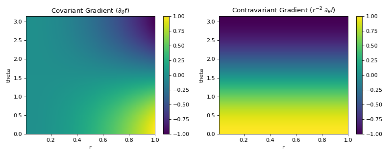
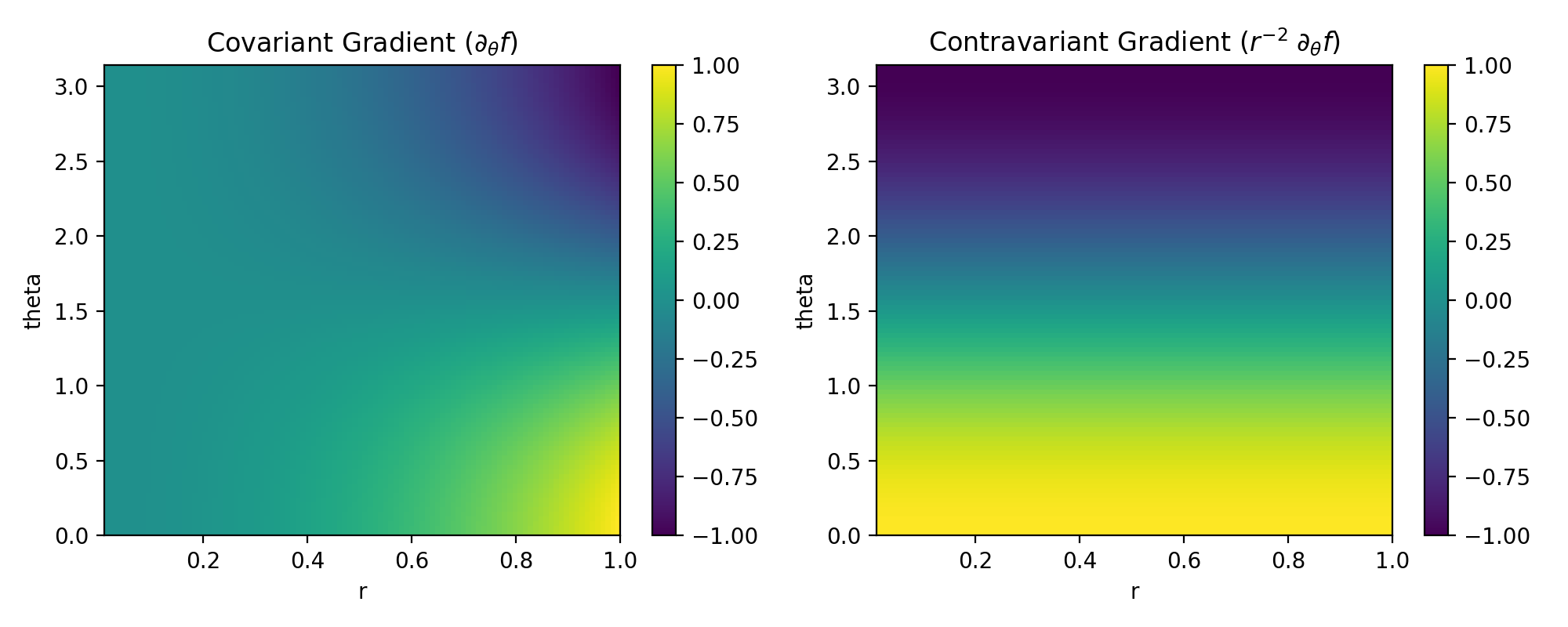
As a demonstration of the difference between covariant and contravariant gradients, let’s consider the gradient in spherical coordinates using the scalar function:
\[f(r, \theta) = r^2 \sin(\theta)\]The gradient is computed in both covariant and contravariant bases. In spherical coordinates, the metric tensor is diagonal:
\[g_{rr} = 1, \quad g_{\theta\theta} = r^2\]and the inverse metric is:
\[g^{rr} = 1, \quad g^{\theta\theta} = \frac{1}{r^2}\]Therefore, the covariant gradient is:
\[\nabla_i f = \left( \frac{\partial f}{\partial r}, \frac{\partial f}{\partial \theta} \right)\]and the contravariant gradient is obtained by raising the index:
\[\nabla^i f = g^{ij} \nabla_j f = \left( \frac{\partial f}{\partial r}, \frac{1}{r^2} \frac{\partial f}{\partial \theta} \right)\]>>> import numpy as np >>> import matplotlib.pyplot as plt >>> from pymetric.differential_geometry.dense_ops import dense_gradient >>> >>> # Create spherical grid >>> r = np.linspace(0.01, 1.0, 100) >>> theta = np.linspace(0, np.pi, 100) >>> R, THETA = np.meshgrid(r, theta, indexing='ij') >>> >>> # Define scalar field f(r, theta) = r^2 * sin(theta) >>> F = R**2 * np.sin(THETA) >>> >>> # Define inverse metric for spherical coordinates >>> IM = np.zeros(R.shape + (2,)) >>> IM[..., 0] = 1 # g^rr = 1 >>> IM[..., 1] = 1 / R**2 # g^thetatheta = 1/r^2 >>> >>> # Compute gradients >>> grad_cov = dense_gradient(F, 0, 2, r, theta, basis='covariant', edge_order=2) >>> grad_contra = dense_gradient(F, 0, 2, r, theta, basis='contravariant', inverse_metric_field=IM, edge_order=2) >>> >>> # Visualize theta component (index 1) of both gradients >>> fig, axes = plt.subplots(1, 2, figsize=(10, 4)) >>> >>> im0 = axes[0].imshow(grad_cov[..., 1].T, origin='lower', extent=[0.01, 1.0, 0, np.pi], aspect='auto') >>> _ = axes[0].set_title(r'Covariant Gradient $(\partial_\theta f)$') >>> _ = fig.colorbar(im0, ax=axes[0]) >>> >>> im1 = axes[1].imshow(grad_contra[..., 1].T, origin='lower', extent=[0.01, 1.0, 0, np.pi], aspect='auto') >>> _ = axes[1].set_title(r'Contravariant Gradient $(r^{-2} \; \partial_\theta f)$') >>> _ = fig.colorbar(im1, ax=axes[1]) >>> >>> for ax in axes: ... _ = ax.set_xlabel("r") ... _ = ax.set_ylabel("theta") >>> >>> plt.tight_layout() >>> plt.show()
(
Source code,png,hires.png,pdf)