differential_geometry.dense_ops.dense_scalar_laplacian_diag#
- differential_geometry.dense_ops.dense_scalar_laplacian_diag(tensor_field: ndarray, Lterm_field: ndarray, inverse_metric_field: ndarray, rank: int, ndim: int, *varargs, field_axes: ndarray | None = None, derivative_axes: ndarray | None = None, out: ndarray | None = None, first_derivative_field: ndarray | None = None, second_derivative_field: ndarray | None = None, edge_order: Literal[1, 2] = 2, **_)[source]#
Compute the element-wise Laplacian of a densely represented tensor field in an orthogonal coordinate system.
This method computes the Laplace-Beltrami operator for a for \(T\):
\[\Delta T = F^\mu \, \partial_\mu T + g^{\mu\mu} \, \partial^2_\mu T,\]where:
\(F^\mu = \frac{1}{\sqrt{|g|}} \, \partial_\mu \sqrt{|g|}\) is the log-derivative of the volume element.
\(g^{\mu\mu}\) is symmetric the inverse metric tensor.
The first term represents the contraction of the F-term and the gradient.
The second term is the contraction of the inverse metric with the Hessian (second derivatives).
Note
This operation is an element-wise operation!
- Parameters:
tensor_field (
numpy.ndarray) –Tensor field of shape
(F_1, ..., F_m, ndim, ...), where the last rank axes are the tensor index dimensions.Hint
Because this function is a low-level callable, it does not enforce the density of the elements in the trailing dimensions of the field. This can be used in some cases where the field is not technically a tensor field.
Lterm_field (
numpy.ndarray) – The F-term field of shape(..., ndim), where the firstmdimensions are broadcast compatible with those oftensor_fieldandinverse_metric_field.inverse_metric_field (
numpy.ndarray) – The inverse metric field of shape(..., ndim), where the firstmdimensions are broadcast compatible with those oftensor_fieldandFterm_field.rank (
int) – Number of trailing axes that represent tensor indices (i.e., tensor rank). The rank determines the number of identified coordinate axes and therefore determines the shape of the returned array.ndim (
int) – The number of total dimensions in the relevant coordinate system. This determines the maximum allowed value formand the number of elements in the trailing dimension of the output.*varargs –
Grid spacing for each spatial axis. Accepts:
A single scalar (applied to all axes),
A list of scalars (one per axis),
A list of coordinate arrays (one per axis),
A mix of scalars and arrays (broadcast-compatible).
If derivative_axes is provided, the number of elements in varargs must match its length. Otherwise, varargs must match the number of spatial dimensions in tensor_field (
m).field_axes (
listofint, optional) –Mapping between each spatial dimension of tensor_field and the corresponding coordinate axis it represents (and therefore the component it represents). field_axes should be a length
msequence of integers between0andndim-1. If not specified, then field_axes is simply0, 1, ..., m-1.Specifying field_axes is critical when working with fields which are incomplete over their spatial domain (missing axes) as field_axes determines how contraction occurs with derivative terms.
derivative_axes (
listofint, optional) –The axes of the tensor_field to perform derivatives over. By default, all
maxes are used when computing derivatives.derivative_axes should be used when certain axes of tensor_field are constant and should be excluded from numerical differentiation. It can also be used when tensor_field has been broadcast to a new set of axes (and therefore has singleton axes) on which differentiation would fail.
first_derivative_field (
numpy.ndarray, optional) –Precomputed first derivatives of the tensor_field with shape
tensor_field.shape + (q,), whereqis the number of axes in derivative_axes or (if the former is not provided), the number of spatial dimensions in tensor_field (m).Specifying first_derivative_field can be used to avoid having to compute the relevant derivatives numerically, which can improve efficiency and accuracy.
second_derivative_field (
numpy.ndarray, optional) –Precomputed second derivatives of the tensor_field with shape
tensor_field.shape + (q,q), whereqis the number of axes in derivative_axes or (if the former is not provided), the number of spatial dimensions in tensor_field (m).Specifying first_derivative_field can be used to avoid having to compute the relevant derivatives numerically, which can improve efficiency and accuracy.
edge_order (
{1, 2}, optional) – Order of accuracy for boundary differences. Default is 2.out (
numpy.ndarray, optional) – An output buffer into which the result should be written. This should be an(..., ndim, ...)array where the leading indices are the broadcasted shape of the spatial components of the tensor_field, Fterm_field, and the inverse_metric_field. The trailing indices must match the non-spatial shape of the tensor_field. If out is not specified, then a new buffer will be created with the correct shape.
- Returns:
Laplacian of tensor_field with shape
tensor_field.shape.- Return type:
Notes
This function assumes a full inverse metric (not diagonal) and uses upper-triangular evaluation of second derivatives to reduce computation using symmetry.
See also
Examples
This example demonstrates computing the Laplace-Beltrami operator for a scalar field in 2D spherical coordinates \((r, \theta)\).
We define the scalar field:
\[\phi(r, \theta) = r^2 \cos(\theta)\]The Laplace-Beltrami operator in spherical coordinates is given by:
\[\Delta \phi = \frac{1}{r^2} \frac{\partial}{\partial r} \left( r^2 \frac{\partial \phi}{\partial r} \right) + \frac{1}{r^2 \sin\theta} \frac{\partial}{\partial \theta} \left( \sin\theta \frac{\partial \phi}{\partial \theta} \right)\]which expands to:
\[\Delta \phi = F^\mu \, \partial_\mu \phi + g^{\mu\nu} \, \partial_\mu \partial_\nu \phi\]where:
\(F^r = \frac{2}{r}\), the derivative of \(\log r^2\)
\(F^\theta = \cot(\theta)\), the derivative of \(\log \sin(\theta)\)
\(g^{rr} = 1\), \(g^{\theta\theta} = \frac{1}{r^2}\) are the components of the inverse metric
>>> import numpy as np
>>> import matplotlib.pyplot as plt
>>> from pymetric.differential_geometry.dense_ops import dense_scalar_laplacian_diag
>>>
>>> # --- Grid in spherical coordinates --- #
>>> r = np.linspace(0.01, 1.0, 100)
>>> theta = np.linspace(0.1, np.pi - 0.1, 100)  # avoid tan(theta)=0
>>> R, THETA = np.meshgrid(r, theta, indexing='ij')
>>>
>>> # --- Scalar field phi(r, theta) = r^2 * cos(theta) --- #
>>> phi = R**2 * np.cos(THETA)
>>>
>>> # --- F-term: [2/r, cot(theta)] --- #
>>> Fterm = np.zeros(R.shape + (2,))
>>> Fterm[:,:,0] = 2 / R
>>> Fterm[:,:,1] = 1 / (R**2 * np.tan(THETA))
>>>
>>> # --- Inverse metric --- #
>>> IM = np.zeros(R.shape + (2,))
>>> IM[..., 0] = 1
>>> IM[..., 1] = 1 / R**2
>>>
>>> # --- Compute Laplacian --- #
>>> lap = dense_scalar_laplacian_diag(phi, Fterm, IM, 0,2,r,theta)
>>>
>>> # --- Plot --- #
>>> _ = plt.imshow(lap.T, origin='lower', extent=[0.01, 1.0, 0.1, np.pi - 0.1], aspect='auto', cmap='viridis')
>>> _ = plt.colorbar(label=r"Laplacian $\Delta \phi$")
>>> _ = plt.title(r"Laplacian of $\phi(r, \theta) = r^2 \cos(\theta)$")
>>> _ = plt.xlabel("r")
>>> _ = plt.ylabel(r"$\theta$")
>>> _ = plt.tight_layout()
>>> plt.show()
(
Source code,png,hires.png,pdf)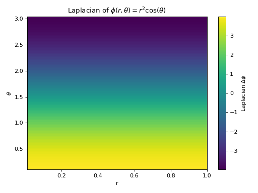