Example Gallery#

Welcome to the PyMetric Example Gallery!

This section showcases a curated collection of concise, self-contained examples demonstrating core features and capabilities of the PyMetric library. Whether you’re exploring differential geometry on structured grids, manipulating tensor fields, or performing symbolic and numerical calculations in curvilinear coordinates, these examples are designed to help you learn by doing.

Each script is:

Minimal and focused on a single concept,
Ready to run and modify interactively,
Accompanied by inline explanations and visual outputs when appropriate.

Browse through, try them out, and use them as starting points for your own work.

Examples are separated by their concept’s location in the codebase.

orphan:

Core Modules: Coordinate Systems #

This gallery highlights examples built around the coordinates module, PyMetric’s foundation for defining and working with structured coordinate systems.

The coordinates module provides a flexible API for defining Cartesian, polar, cylindrical, spherical, and general curvilinear systems, as well as custom user-defined coordinates. These examples showcase how to:

Instantiate and explore predefined coordinate systems,
Evaluate coordinate transforms and Jacobians,
Work with symbolic metrics and basis vectors,
Integrate coordinate systems into grid construction and field definitions.

Whether you’re visualizing a spherical metric or customizing an orthogonal system for a simulation, these examples serve as practical guides to mastering the geometry backbone of PyMetric.

Hint

For in-depth user documentation, see Coordinate Systems: General Info.

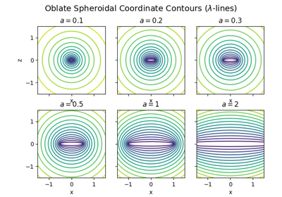
Oblate Spheroidal Coordinates: Effect of Eccentricity

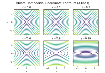
Oblate Homoeoidal Coordinates: Effect of Eccentricity

orphan:

Core Modules: Grids #

This gallery highlights examples built around the grids module, which provides the structured backbone for numerical field representation and finite-difference computation in PyMetric.

The grids module offers a powerful API for constructing regular, scaled, and fully generic structured grids—each integrated with coordinate system metadata and axis-aware utilities. These examples demonstrate how to:

Create uniform and non-uniform spatial grids tied to coordinate systems,
Extract coordinate arrays and physical units,
Use ghost zones, chunking, and broadcasting,
Apply field operations like partial derivatives and interpolation.

Whether you’re building a finite-difference solver or managing multi-axis tensor data, these examples provide practical insight into leveraging PyMetric’s spatial grid machinery.

Hint

For detailed user documentation, see Geometric Grids: General Info.

Cartesian Gradient (Non-Uniform)

Grid Laplacian

orphan:

Core Modules: Fields #

This gallery showcases examples based on the fields module, PyMetric’s core abstraction for physical quantities defined over space—scalars, vectors, tensors, and more.

The fields module provides a unified interface for working with field components, units, buffers, and coordinate-aware differential operations. These examples walk through how to:

Construct scalar, vector, and tensor fields over structured grids,
Manage physical units and buffer types (e.g., NumPy, unyt, HDF5),
Broadcast, expand, reduce, and reshape field components,
Apply differential geometry operations like gradients, divergence, and Laplacians,
Combine symbolic metadata with numerical buffers for hybrid workflows.

From initializing a field from an analytic expression to computing its divergence in curved space, these examples demonstrate the expressive and extensible field API at the heart of PyMetric.

Hint

For complete documentation, see Fields: Overview.