differential_geometry.dense_utils.dense_raise_index

differential_geometry.dense_utils.dense_raise_index(tensor_field: ndarray, index: int, rank: int, inverse_metric_field: ndarray, out: ndarray | None = None, **kwargs) → ndarray

Raise a specified index of a tensor field using the inverse metric tensor.

Parameters:

• tensor_field (numpy.ndarray) –

  The tensor field whose index signature is to be adjusted. The array should have shape (F₁, ..., F_m, I₁, ..., I_r), where:

  • (F₁, ..., F_m) are the field (spatial or grid) dimensions,

  • (I₁, ..., I_r) are the tensor index dimensions, and

  • r is the tensor rank (i.e., the number of tensor indices, inferred from tensor_signature).

• index (int) – The index to lower, ranging from 0 to rank-1.

• rank (int) – The tensor rank (number of tensor indices, not including grid dimensions).

• inverse_metric_field (numpy.ndarray, optional) –

  The inverse metric tensor used to raise covariant indices. This can be either:

  • A full inverse metric of shape (…, N, N), or

  • A diagonal inverse metric of shape (…, N).

  Must match the metric type (diagonal vs full) and be broadcast-compatible with tensor_field.

• out (numpy.ndarray, optional) – Optional output array to store the result. If provided, must have the same shape and dtype as the expected output, and will be used for in-place storage.

Returns:

A tensor field with the specified index raised. Has the same shape as tensor_field.

Return type:

numpy.ndarray

See also

dense_lower_index, dense_adjust_tensor_signature

Raises:

ValueError – If the input shapes or indices are invalid.

Examples

In spherical coordinates, if you have a covariant vector:

\[{\bf v} = r {\bf e}^\theta\]

Then the contravariant version is:

\[v^\theta = g^{\theta \mu} v_\mu = g^{\theta \theta} v_\theta = \frac{1}{r^2} v_{\theta} = \frac{1}{r}.\]

Let’s see this work in practice:

>>> import numpy as np
>>> from pymetric.differential_geometry.dense_utils import dense_raise_index
>>>
>>> # Construct the vector field at a point.
>>> # We'll need the metric (inverse) and the vector field at the point.
>>> r,theta = 2,np.pi/4
>>> v_cov = np.asarray([0,r,0])
>>>
>>> # Construct the metric tensor.
>>> g_inv = np.diag([1, 1 / r**2, 1 / (r**2 * np.sin(theta)**2)])
>>>
>>> # Now we can use the inverse metric to raise the tensor index.
>>> dense_raise_index(v_cov, index=0, rank=1, inverse_metric_field=g_inv)
array([0. , 0.5, 0. ])

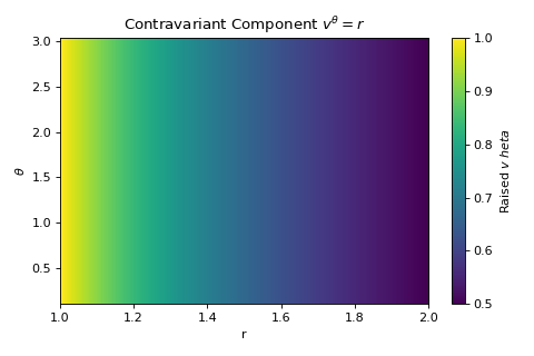
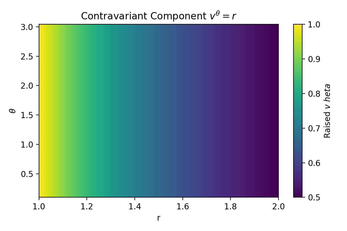
A 2D example on a spherical grid:

>>> import numpy as np
>>> import matplotlib.pyplot as plt
>>> from pymetric.differential_geometry.dense_utils import dense_raise_index
>>>
>>> # Define 2D spherical grid
>>> r = np.linspace(1, 2, 100)
>>> theta = np.linspace(0.1, np.pi - 0.1, 100)
>>> R, THETA = np.meshgrid(r, theta, indexing="ij")
>>>
>>> # Define a covariant vector field: v_θ = R
>>> v_cov = np.zeros(R.shape + (2,))
>>> v_cov[..., 1] = R  # non-zero only in theta direction
>>>
>>> # Define the inverse metric: g^{rr} = 1, g^{θθ} = 1 / r^2
>>> g_inv = np.zeros(R.shape + (2,))
>>> g_inv[..., 0] = 1
>>> g_inv[..., 1] = 1 / R**2
>>>
>>> # Raise the index
>>> v_contra = dense_raise_index(v_cov, index=0, rank=1, inverse_metric_field=g_inv)
>>>
>>> # Plot the raised θ-component
>>> _ = plt.figure(figsize=(6, 4))
>>> im = plt.imshow(v_contra[..., 1].T, extent=[1, 2, 0.1, np.pi - 0.1], aspect="auto", origin="lower")
>>> _ = plt.colorbar(im, label="Raised $v^\theta$")
>>> _ = plt.xlabel("r")
>>> _ = plt.ylabel(r"$\theta$")
>>> _ = plt.title(r"Contravariant Component $v^\theta = r$")
>>> _ = plt.tight_layout()
>>> _ = plt.show()

(Source code, png, hires.png, pdf)