differential_geometry.dense_ops.dense_gradient_covariant#
- differential_geometry.dense_ops.dense_gradient_covariant(tensor_field: ndarray, rank: int, ndim: int, *varargs, field_axes: Sequence[int] | None = None, output_indices: Sequence[int] | None = None, edge_order: Literal[1, 2] = 2, out: _Buffer | _SupportsArray[dtype[Any]] | _NestedSequence[_SupportsArray[dtype[Any]]] | complex | bytes | str | _NestedSequence[complex | bytes | str] | None = None, **_) ndarray[source]#
Compute the element-wise covariant gradient of a tensor field.
This function computes the raw partial derivatives \(\partial_\mu T\) of a tensor (or array) field with respect to its grid coordinates, treating each tensor component independently.
It returns the gradient along all spatial axes (or a subset, if specified), storing results in the final axis of the output. This is the covariant gradient in the sense of component-wise partial derivatives, without applying connection terms (i.e., no Christoffel symbols). It is not the covariant derivative.
Warning
This is a low-level utility function. It does not validate input shapes or ensure coordinate consistency. It assumes that the tensor rank and grid structure are correct.
- Parameters:
tensor_field (
numpy.ndarray) –Tensor field of shape
(F_1, ..., F_m, N, ...), where the last rank axes are the tensor index dimensions. The partial derivatives are computed over the first m axes.Hint
Because this function is a low-level callable, it does not enforce the density of the elements in the trailing dimensions of the field. This can be used in some cases where the field is not technically a tensor field.
rank (
int) – Number of trailing axes that represent tensor indices (i.e., tensor rank). The rank determines the number of identified coordinate axes and therefore determines the shape of the returned array.ndim (
int) – The number of total dimensions in the relevant coordinate system. This determines the maximum allowed value formand the number of elements in the trailing dimension of the output.*varargs –
Grid spacing for each spatial axis. Follows the same format as
numpy.gradient(), and can be:A single scalar (applied to all spatial axes),
A list of scalars (one per axis),
A list of coordinate arrays (one per axis),
A mix of scalars and arrays (broadcast-compatible).
If field_axes is provided, varargs must match its length. If axes is not provided, then varargs should be
tensor_field.ndim - rankin length (or be a scalar).field_axes (
listofint, optional) – The spatial axes over which to compute the component-wise partial derivatives. If field_axes is not specified, then alltensor_field.ndim - rankaxes are computed.output_indices (
listofint, optional) –Explicit mapping from each axis listed in field_axes to the indices in the output’s final dimension of size
ndim. This parameter allows precise control over the placement of computed gradients within the output array.If provided, output_indices must have the same length as field_axes. Each computed gradient along the spatial axis
field_axes[i]will be stored at indexoutput_indices[i]in the last dimension of the output.If omitted, the default behavior is
output_indices = field_axes, i.e., gradients are placed in the output slot corresponding to their source axis.Note
All positions in the final axis of the output array not listed in
output_indicesare left unmodified (typically zero-filled unlessoutwas pre-populated).edge_order (
{1, 2}, optional) – Gradient is calculated using N-th order accurate differences at the boundaries. Default: 1.out (
numpy.ndarray, optional) – Buffer in which to store the output to preserve memory. If provided, out must have shapetensor_field.shape + (ndim,). If out is not specified, then it is allocated during the function call.
- Return type:
See also
numpy.gradientThe computational backend for this operation.
dense_gradient_contravariant_fullContravariant gradient for full metric.
dense_gradient_contravariant_diagContravariant gradient for diagonal metric.
dense_gradientWrapper for user-facing gradient computations.
Examples
In a simple 1-D case, we can use this function to compute the gradient.
>>> import numpy as np
>>> from pymetric.differential_geometry.dense_ops import (
...     dense_gradient_covariant,
... )
>>>
>>> x = np.linspace(0, 4, 5)          #  [0, 1, 2, 3, 4]
>>> f = x**2                          #  [0, 1, 4, 9, 16]
>>>
>>> grad_cov = dense_gradient_covariant(f, 0, 1, 1.0)          # dx = 1
>>> grad_cov
array([[0.],
       [2.],
       [4.],
       [6.],
       [8.]])
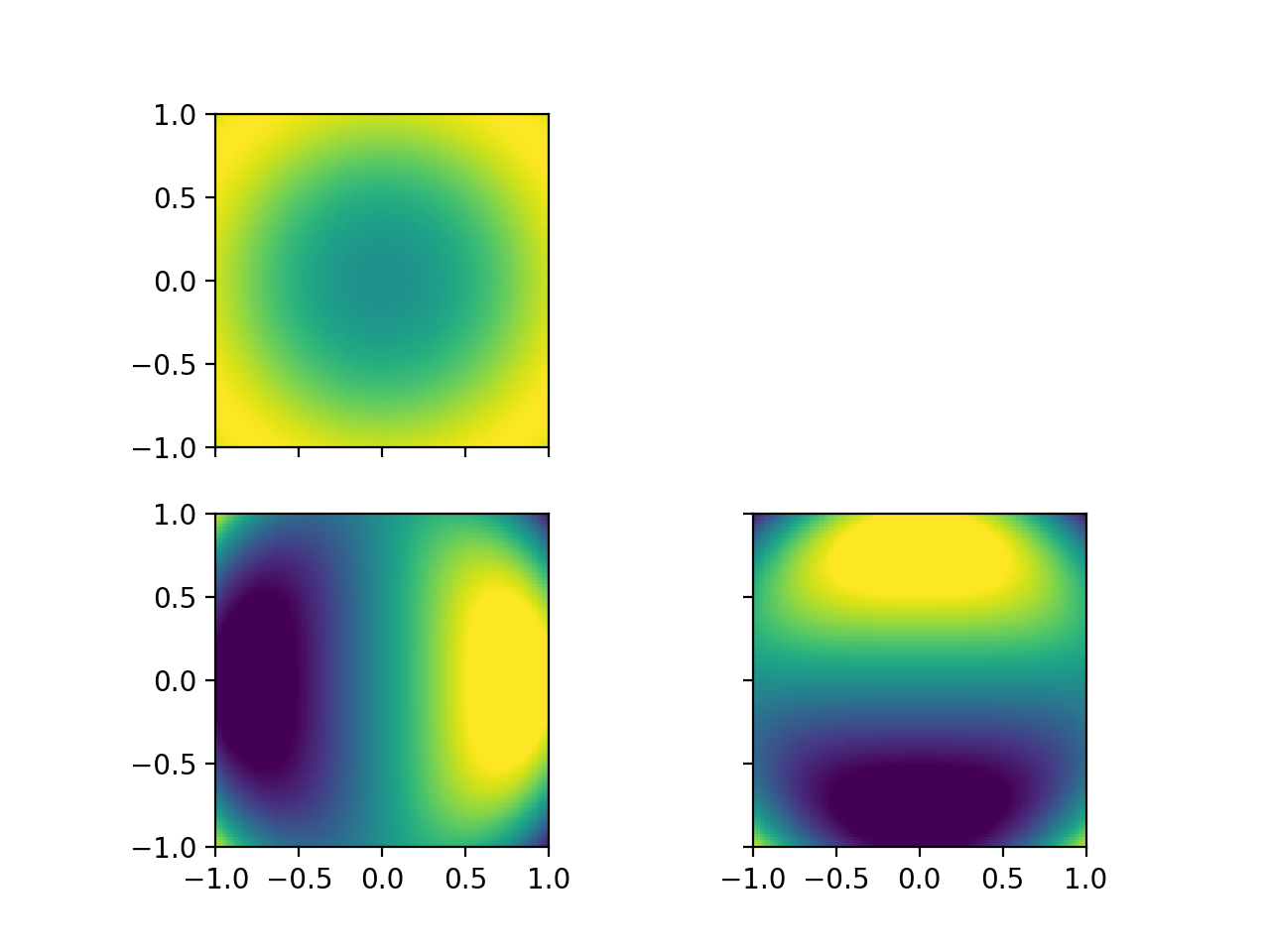
In a more complicated 2-D case, the call sequence still looks the same.
>>> import numpy as np
>>> from pymetric.differential_geometry.dense_ops import dense_gradient_covariant
>>> import matplotlib.pyplot as plt
>>>
>>> x = np.linspace(-1,1,100)
>>> y = np.linspace(-1,1,100)
>>> X,Y = np.meshgrid(x,y)
>>> Z = np.sin(X**2 + Y**2)
>>>
>>> grad = dense_gradient_covariant(Z,0,2,x,y)
>>>
>>> fig,axes = plt.subplots(2,2,sharex=True,sharey=True)
>>> axes[0,1].set_visible(False)
>>> _ = axes[0,0].imshow(Z.T, origin='lower', vmin=-1,vmax=1,extent=(-1,1,-1,1))
>>> _ = axes[1,0].imshow(grad[...,0].T, origin='lower', vmin=-1,vmax=1,extent=(-1,1,-1,1))
>>> _ = axes[1,1].imshow(grad[...,1].T, origin='lower', vmin=-1,vmax=1,extent=(-1,1,-1,1))
>>> _ = plt.show()
(
Source code,png,hires.png,pdf)