Cartesian Gradient (Non-Uniform)

Compute gradients in a Cartesian coordinate system on a non-uniform grid with higher resolution near the origin.

This example demonstrates how to compute gradients in a Cartesian coordinate system using a non-uniform grid that provides higher resolution near the origin and sparser coverage near the domain boundaries.

We use PyMetric’s geometric grid abstractions to handle the complexities of computing numerical derivatives over irregularly spaced points. In particular, this example highlights:

• The use of GenericGrid for non-uniform grids,

• Accurate gradient computation via dense_gradient(),

• Comparison of numerical and analytical gradients in Cartesian coordinates.

Such workflows are particularly useful in simulations where local resolution is needed around a feature of interest (e.g., boundary layers, shock fronts, or potential wells), without sacrificing performance over the full domain.

Coordinate Setup

The first thing to do is to create the coordinate system. For this example, we’re going to use a cartesian coordinate system in 2D: CartesianCoordinateSystem2D.

import matplotlib.pyplot as plt
import numpy as np
from matplotlib.colors import LogNorm

# sphinx_gallery_thumbnail_number = 3
from pymetric import CartesianCoordinateSystem2D, GenericGrid

# Create the coordinate system. We don't need
# any parameters for this one.
csys = CartesianCoordinateSystem2D()

Build a Non-Uniform Grid

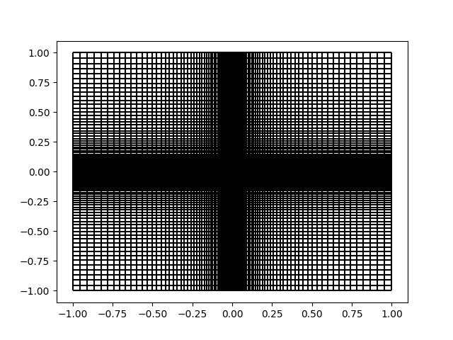
For this operation, we’d like to have a grid with points clustered around the origin and with lower resolution near the outskirts. One simple prescription for this is the use of the \(\tanh\) transformation, which will nicely produce this behavior.

# Define a tanh streching function.
def tanh_scale(num_points, x0, x1, s=1):
    # Create linear spacing from -1 -> 1.
    u = np.linspace(-1, 1, num_points)
    u_stretched = np.sign(u) * (np.abs(u) ** s)
    return x0 + (x1 - x0) * (u_stretched + 1) / 2


# Generate 2D coordinates
x = tanh_scale(128, -1, 1, s=3)
y = tanh_scale(128, -1, 1, s=3)

# Define the bounding box for the coordinate domain
bbox = [[-1, -1], [1, 1]]

# Create the grid
grid = GenericGrid(csys, [x, y], bbox=bbox, center="cell")

A nice feature of PyMetric grids is that you can easily visualize slices of them using the plot_grid_lines() function. We can do that here to validate that we have achieved our intentions:

fig, ax = plt.subplots(1, 1)
grid.plot_grid_lines(include_ghosts=True, ax=ax)
plt.show()

Define the Field

We’ll now define a scalar field over this grid to test the gradient computation. Specifically, we define:

\[\Phi(x, y) = \sin\left[aR^2\right],\; R^2 = x^2 + y^2\]

where \(a\) is a tunable frequency parameter. The analytical gradient is

\[\begin{split}\nabla_i \Phi = \begin{bmatrix}2ax \cos(a R^2)\\2ay\cos(aR^2)\end{bmatrix}\end{split}\]

a = 5.0  # Frequency parameter

# Generate meshgrid from the grid
X, Y = grid.compute_domain_mesh(axes=["x", "y"])
R2 = X**2 + Y**2
Phi = np.sin(a * R2)

# Plot the scalar field
fig, ax = plt.subplots()
c = ax.pcolormesh(X, Y, Phi, shading="auto", cmap="viridis")
fig.colorbar(c, ax=ax, label=r"$\Phi(x, y)$")
ax.set_aspect("equal")
ax.set_title(r"Scalar Field $\Phi = \sin[a(x^2 + y^2)]$")
plt.show()

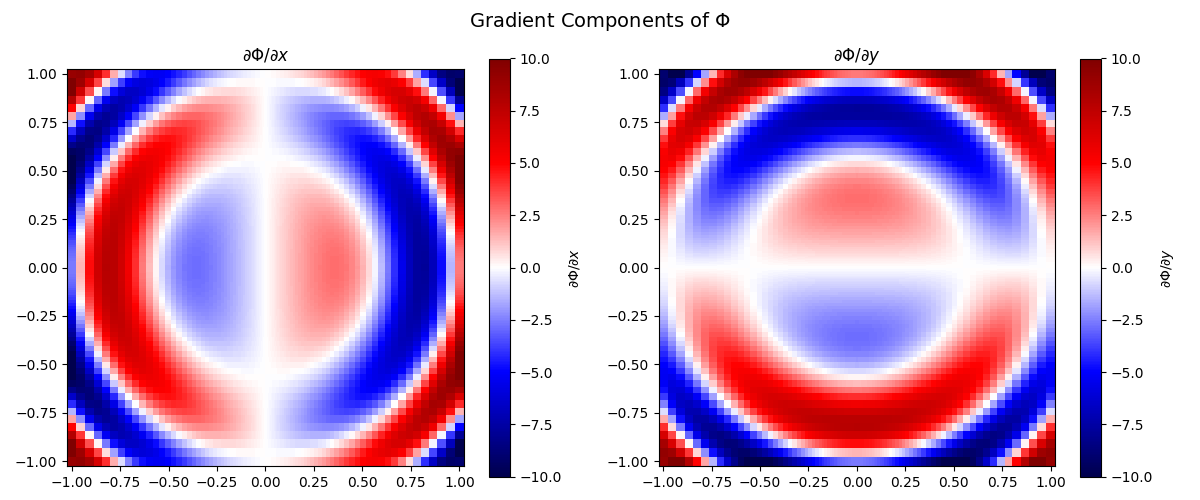
Compute the Gradient

Now we’ll compute the gradient of the field numerically using PyMetric’s grid interface. This computes:

\[\nabla \Phi = \left[ \frac{\partial \Phi}{\partial x}, \frac{\partial \Phi}{\partial y} \right]\]

grad = grid.dense_gradient(Phi, ["x", "y"], edge_order=2)

# Plot the gradient components
fig, axes = plt.subplots(1, 2, figsize=(12, 5))
labels = [r"$\partial \Phi / \partial x$", r"$\partial \Phi / \partial y$"]

for i, ax in enumerate(axes):
    c = ax.pcolormesh(
        X, Y, grad[..., i], shading="auto", cmap="seismic", vmin=-10, vmax=10
    )
    fig.colorbar(c, ax=ax, label=labels[i])
    ax.set_title(labels[i])
    ax.set_aspect("equal")

plt.suptitle(r"Gradient Components of $\Phi$", fontsize=14)
plt.tight_layout()
plt.show()

Compare with Analytical Gradient

The analytical gradient is:

\[\begin{split}\nabla_i \Phi = \begin{bmatrix}2ax \cos(a R^2)\\2ay\cos(aR^2)\end{bmatrix}\end{split}\]

dPhi_dx_exact = 2 * a * X * np.cos(a * R2)
dPhi_dy_exact = 2 * a * Y * np.cos(a * R2)

# Compute error
err_x = np.abs((grad[..., 0] - dPhi_dx_exact) / dPhi_dx_exact)
err_y = np.abs((grad[..., 1] - dPhi_dy_exact) / dPhi_dy_exact)

print(f"Mean relative error: {np.mean(err_x)},{np.mean(err_y)}.")

# Plot errors
fig, axes = plt.subplots(1, 2, figsize=(12, 5))
titles = [r"$\partial \Phi / \partial x$ Error", r"$\partial \Phi / \partial y$ Error"]
errors = [err_x, err_y]

for i, ax in enumerate(axes):
    c = ax.pcolormesh(
        X,
        Y,
        errors[i],
        shading="auto",
        cmap="binary",
        norm=LogNorm(vmax=0.1, vmin=1e-7),
    )
    fig.colorbar(c, ax=ax)
    ax.set_title(titles[i])
    ax.set_aspect("equal")

plt.suptitle(
    r"Gradient Relative Error (Numerical - Analytical)/Analytical", fontsize=14
)
plt.tight_layout()
plt.show()

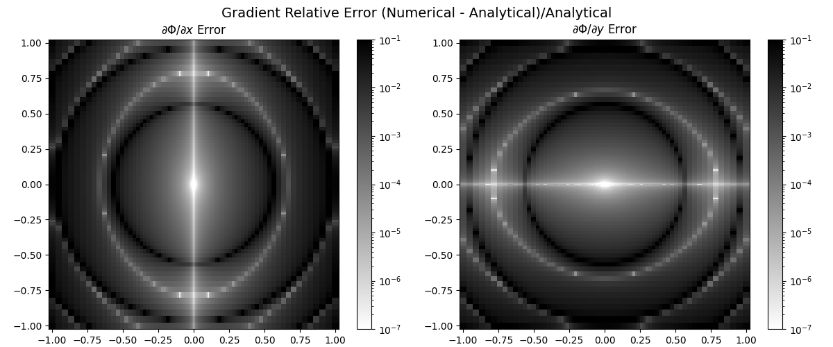
Mean relative error: 0.014364471045282894,0.014364471045282892.