Gradient In Cartesian Coordinates

Calculate the gradient of a function in Cartesian coordinates.

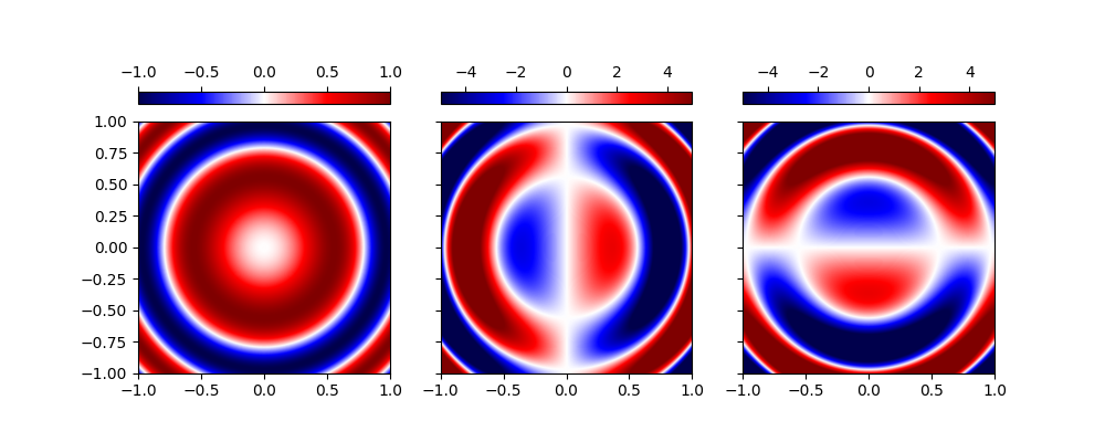
In this example, we’ll use the methods in the low-level differential_geometry to compute the gradient of the function

\[f(x_1,x_2) = A\sin\left(\omega \left[x_1^2+x_2^2\right]\right).\]

In Cartesian coordinates, this is an extremely simple operation to compute directly:

\[\nabla_i f(x_1,x_2) = 2\omega x_i f(x_1,x_2).\]

To do this computationally, we need to perform the following operations:

import matplotlib.pyplot as plt

# Import necessary modules.
import numpy as np

from pymetric.differential_geometry.dense_ops import dense_gradient

# Settings:
A, omega = 1, 5
cmap = "seismic"

# Create the x and y grids.
x, y = np.linspace(-1, 1, 500), np.linspace(-1, 1, 500)
X, Y = np.meshgrid(x, y, indexing="ij")

# Compute the field `Z`
R = X**2 + Y**2
Z = A * np.sin(omega * R)

# Compute the gradient.
gradZ = dense_gradient(Z, 0, 2, x, y)

With the gradient computed, we can plot the output. The result has a shape (500,500,2).

fig, ax = plt.subplots(1, 3, figsize=(10, 4), sharex=True, sharey=True)

ax[0].imshow(Z.T, extent=[-1, 1, -1, 1], cmap=cmap, vmin=-A, vmax=A)
ax[1].imshow(
    gradZ[..., 0].T, extent=[-1, 1, -1, 1], cmap=cmap, vmin=-A * omega, vmax=A * omega
)
ax[2].imshow(
    gradZ[..., 1].T, extent=[-1, 1, -1, 1], cmap=cmap, vmin=-A * omega, vmax=A * omega
)

plt.colorbar(
    plt.cm.ScalarMappable(plt.Normalize(vmin=-A, vmax=A), cmap=cmap),
    ax=ax[0],
    orientation="horizontal",
    location="top",
)
plt.colorbar(
    plt.cm.ScalarMappable(plt.Normalize(vmin=-A * omega, vmax=A * omega), cmap=cmap),
    ax=ax[1],
    orientation="horizontal",
    location="top",
)
plt.colorbar(
    plt.cm.ScalarMappable(plt.Normalize(vmin=-A * omega, vmax=A * omega), cmap=cmap),
    ax=ax[2],
    orientation="horizontal",
    location="top",
)

plt.show()