Elementwise Partial Derivative (2D Cosine)

This example demonstrates how to compute the elementwise partial derivatives of a scalar field in a Cartesian coordinate system using PyMetric’s high-level DenseField interface.

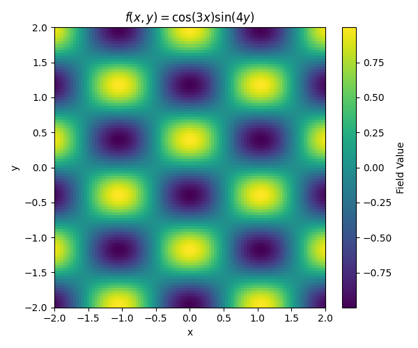
We define a scalar field of the form:

\[f(x, y) = \cos(3x)\sin(4y)\]

We then compute and visualize:

• The original scalar field

• The partial derivative with respect to \(x\)

• The partial derivative with respect to \(y\)

This is useful for verifying numerical derivative accuracy in simple geometries.

Dependencies

• DenseField

• UniformGrid

• CartesianCoordinateSystem2D

import matplotlib.pyplot as plt
import numpy as np

Import required modules

from pymetric import CartesianCoordinateSystem2D, DenseField, UniformGrid

Setup the coordinate system and uniform grid

cs = CartesianCoordinateSystem2D()

# Define bounding box and resolution
bbox = [[-2, -2], [2, 2]]
grid = UniformGrid(cs, bbox, [100, 100], center="cell")

Define the scalar field on the grid

We define f(x, y) = cos(3x) * sin(4y)

field: DenseField = DenseField.from_function(
    lambda x, y: np.cos(3 * x) * np.sin(4 * y), grid, axes=["x", "y"]
)

# Extract mesh for plotting
X, Y = field.grid.compute_domain_mesh(axes=["x", "y"])

Plot the original scalar field

plt.figure(figsize=(6, 5))
plt.pcolormesh(X, Y, field[...], shading="auto", cmap="viridis")
plt.title(r"$f(x, y) = \cos(3x)\sin(4y)$")
plt.xlabel("x")
plt.ylabel("y")
plt.colorbar(label="Field Value")
plt.tight_layout()
plt.show()

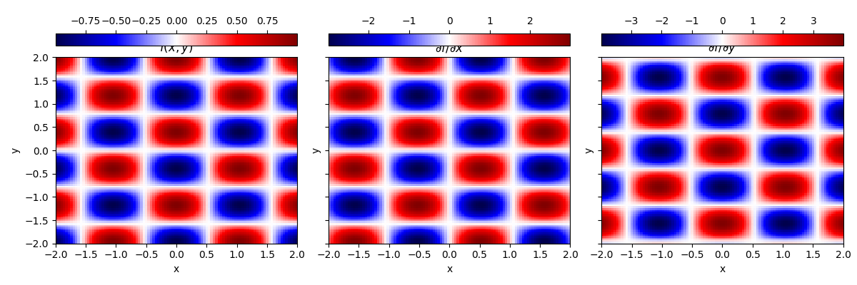
Compute and plot the partial derivatives

Use the element_wise_partial_derivative method from DenseField.

gradF = field.element_wise_partial_derivatives()

# Create the subplots
fig, axes = plt.subplots(1, 3, figsize=(12, 4), sharex=True, sharey=True)

# Plot original field
a = axes[0].pcolormesh(X, Y, field[...], shading="auto", cmap="seismic")
axes[0].set_title(r"$f(x, y)$")
plt.colorbar(a, ax=axes[0], location="top", orientation="horizontal")

# Partial w.r.t x
b = axes[1].pcolormesh(X, Y, gradF[..., 0], shading="auto", cmap="seismic")
axes[1].set_title(r"$\partial f / \partial x$")
plt.colorbar(b, ax=axes[1], location="top", orientation="horizontal")

# Partial w.r.t y
c = axes[2].pcolormesh(X, Y, gradF[..., 1], shading="auto", cmap="seismic")
axes[2].set_title(r"$\partial f / \partial y$")
plt.colorbar(c, ax=axes[2], location="top", orientation="horizontal")

for ax in axes:
    ax.set_xlabel("x")
    ax.set_ylabel("y")

plt.tight_layout()
plt.show()