NFW Density from Potential

Compute the NFW density from a potential profile.

This example demonstrates how to compute the dark matter density profile of a Navarro–Frenk–White (NFW) halo by applying the Laplacian operator to its gravitational potential in spherical coordinates.

We use the Poisson equation to numerically recover the NFW density profile:

\[\nabla^2 \Phi = 4\pi G \rho\]

Given the analytic form of the NFW potential \(\Phi(r)\), we compute the Laplacian numerically using PyMetric and compare the inferred density \(\rho(r)\) to its known analytic form.

import matplotlib.pyplot as plt

# Imports
import numpy as np

from pymetric import DenseField, GenericGrid, SphericalCoordinateSystem

# Characteristic density and scale radius for the NFW profile
rho0 = 1.0
Rs = 1.0

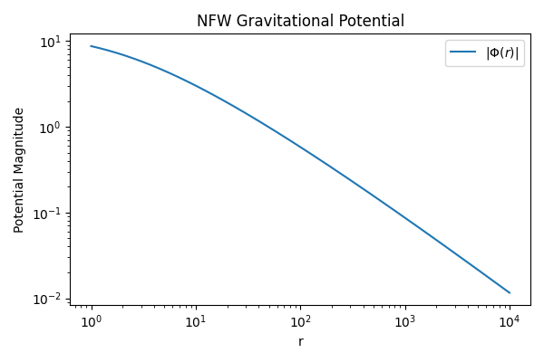
Define the NFW gravitational potential.

\[\Phi(r) = -\frac{4\pi G \rho_0 R_s^3}{r} \log\left(1 + \frac{r}{R_s}\right)\]

def nfw_potential(r, _rho0=rho0, _Rs=Rs):
    return -(4 * np.pi * _rho0 * _Rs**3 / r) * np.log(1 + r / _Rs)

Define the analytic NFW density profile derived from the Poisson equation.

\[\rho(r) = \frac{\rho_0}{\left(\frac{r}{R_s}\right)(1 + \frac{r}{R_s})^2}\]

def nfw_density(r, _rho0=rho0, _Rs=Rs):
    xi = r / _Rs
    return _rho0 / (xi * (1 + xi) ** 2)

Setup the grid using a spherical coordinate system.

We use high radial resolution to accurately capture structure in \(r\), and minimal angular resolution since the profile is spherically symmetric.

csys = SphericalCoordinateSystem()

r_coord = np.geomspace(1.0, 1e4, 3000)
theta_coord = np.linspace(0, np.pi, 10)
phi_coord = np.linspace(0, 2 * np.pi, 10)

grid = GenericGrid(csys, [r_coord, theta_coord, phi_coord], center="vertex")
grid.fill_values = {"r": 1, "theta": 1, "phi": 1}  # handle r=0 and boundaries safely

Evaluate the NFW potential on the grid.

field: DenseField = DenseField.from_function(nfw_potential, grid, axes=["r"])

Visualize the magnitude of the potential vs radius.

plt.figure(figsize=(6, 4))
plt.loglog(r_coord, np.abs(field[...]), label=r"$|\Phi(r)|$")
plt.xlabel("r")
plt.ylabel("Potential Magnitude")
plt.title("NFW Gravitational Potential")
plt.legend()
plt.tight_layout()
plt.show()

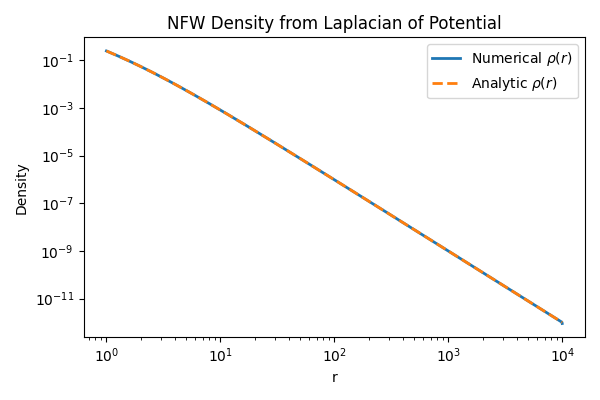
Compute the numerical Laplacian of the field and infer the density using:

\[\rho(r) = \frac{1}{4\pi G} \nabla^2 \Phi\]

laplacian = field.element_wise_laplacian()
numerical_density = laplacian[...] / (4 * np.pi)

Compare the numerical density to the analytic NFW density profile.

plt.figure(figsize=(6, 4))
plt.loglog(r_coord, numerical_density, label="Numerical $\\rho(r)$", lw=2)
plt.loglog(r_coord, nfw_density(r_coord), "--", label="Analytic $\\rho(r)$", lw=2)
plt.xlabel("r")
plt.ylabel("Density")
plt.title("NFW Density from Laplacian of Potential")
plt.legend()
plt.tight_layout()
plt.show()