NFW Density in Oblate Coordinates

Compute an NFW density in Oblate Coordinates.

This example demonstrates how to compute the dark matter density profile of a Navarro–Frenk–White (NFW) halo using the Laplacian of its gravitational potential in an oblate homoeoidal coordinate system.

We use the Poisson equation:

\[\nabla^2 \Phi = 4 \pi G \rho\]

to infer the density \(\rho(r)\) numerically and compare the results to the analytic NFW solution, validating PyMetric’s support for oblate curvilinear coordinates.

import matplotlib.pyplot as plt

Imports and Parameters

We start by importing necessary libraries and defining physical and coordinate parameters.

import numpy as np
from matplotlib.colors import AsinhNorm, LogNorm

from pymetric import DenseField, GenericGrid, OblateHomoeoidalCoordinateSystem

# Global parameters for the NFW profile
rho0 = 1.0  # Characteristic density
Rs = 100  # Scale radius
ecc = 0.6  # Eccentricity of the oblate coordinate system

# Coordinate bounds and resolution
bbox = [[-1, 0, 0], [1e4, np.pi, 2 * np.pi]]
r = np.geomspace(1e-1, 9.9e3, 500)  # Radial coordinate
theta = np.linspace(1e-2, np.pi - 1e-2, 500)  # Polar angle (avoid poles)
phi = np.linspace(1e-2, 2 * np.pi - 1e-2, 500)  # Azimuthal angle

Define the Gravitational Potential

The NFW potential is given by:

\[\Phi(r) = -\frac{4\pi G \rho_0 R_s^3}{r} \log\left(1 + \frac{r}{R_s}\right)\]

This is defined only in terms of the radial coordinate \(r\).

def nfw_potential(r, _rho0=rho0, _Rs=Rs):
    """NFW gravitational potential Φ(r)."""
    return -(4 * np.pi * _rho0 * _Rs**3 / r) * np.log(1 + r / _Rs)

The analytic NFW density is:

\[\rho(r) = \frac{\rho_0}{(r/R_s)(1 + r/R_s)^2}\]

We’ll use this for validating our numerical result.

def nfw_density_spherical(r, _rho0=rho0, _Rs=Rs):
    """Analytic density ρ(r) for a spherical NFW halo."""
    xi = r / _Rs
    return _rho0 / (xi * (1 + xi) ** 2)

Construct Coordinate System and Grid

We define an oblate homoeoidal coordinate system with a given eccentricity. The computational grid is constructed over three axes:

• \(\xi\) (a radial-like coordinate aligned with the symmetry axis)

• \(\theta\) (the polar angle)

• \(\phi\) (the azimuthal angle)

The coordinate system is embedded in 3D, and the transformation from Cartesian coordinates introduces singularities at certain angular positions.

Important

This coordinate system has a metric singularity at \(\theta = 0\) and \(\theta = \pi\), which can lead to undefined behavior in numerical operations such as computing derivatives or applying the Laplacian if values at those points are needed but not explicitly provided.

To safely evaluate expressions over a subset of axes (e.g., computing a Laplacian over only \(\xi\) and \(\theta\)), we provide default fill values for missing dimensions:

grid.fill_values = {"xi": 1, "theta": 1, "phi": 1}

This tells PyMetric to use fixed representative values for unspecified axes (e.g., holding \(\phi=1\) constant if it’s not one of the axes being operated on). This is especially important when the metric or differential operators implicitly require coordinate values from all axes.

Choosing theta=1 ensures we avoid the singular axis at \(\theta = 0\), which would otherwise cause issues during evaluation of geometric quantities like the metric tensor.

cs = OblateHomoeoidalCoordinateSystem(ecc=ecc)
grid = GenericGrid(cs, [r, theta, phi], bbox=bbox, center="cell")

# Provide default values for unused axes during partial operations.
grid.fill_values = {
    "xi": 1,  # mid-range reference radius
    "theta": 1,  # avoids θ = 0 or π
    "phi": 1,  # arbitrary fixed azimuth
}

Evaluate the Potential on the Grid

We now evaluate the potential over the grid by sampling it along the radial direction. This is done with from_function().

field = DenseField.from_function(nfw_potential, grid, axes=["xi"])

Compute Laplacian and Infer Density

Using the Poisson equation, we convert the numerical Laplacian into a density field:

\[\rho = \frac{1}{4\pi G} \nabla^2 \Phi\]

(with \(G = 1\) in our units).

lap = field.element_wise_laplacian(output_axes=["xi", "theta"])
density_field = lap / (4 * np.pi)

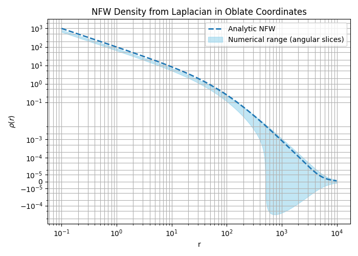
We collapse angular variations in the density by taking the min and max over angular slices, and compare this envelope to the spherical analytic profile.

Depending on the values for the eccentricity and the profile parameters, you may notice that the density can be negative! In fact, this is not a glitch or bug, it is a result about the validity of the NFW profile in this coordinate system.

min_density = np.min(density_field.as_array(), axis=1)
max_density = np.max(density_field.as_array(), axis=1)
ref_density = nfw_density_spherical(r)

plt.figure(figsize=(7, 5))
plt.plot(r, ref_density, "--", lw=2, label="Analytic NFW")
plt.fill_between(
    r,
    min_density,
    max_density,
    color="skyblue",
    alpha=0.5,
    label="Numerical range (angular slices)",
)
plt.xlabel("r")
plt.ylabel(r"$\rho(r)$")
plt.title("NFW Density from Laplacian in Oblate Coordinates")
plt.legend()
plt.grid(True, which="both")
plt.yscale("asinh", linear_width=1e-5)
plt.xscale("log")
plt.tight_layout()
plt.show()

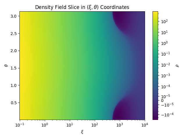
We’ll now plot the full 2D slice of the computed density field in \((\xi, \theta)\) space. This will help to illustrate the points at which the profile becomes negative. Notably, this is most relevant at the poles!

XI, THETA = grid.compute_domain_mesh(axes=["xi", "theta"])
c = plt.pcolormesh(XI, THETA, density_field[...], norm=AsinhNorm(linear_width=1e-5))
plt.xscale("log")
plt.xlabel(r"$\xi$")
plt.ylabel(r"$\theta$")
plt.colorbar(c, label=r"$\rho$")
plt.title(r"Density Field Slice in $(\xi, \theta)$ Coordinates")
plt.tight_layout()
plt.show()

Interpolation

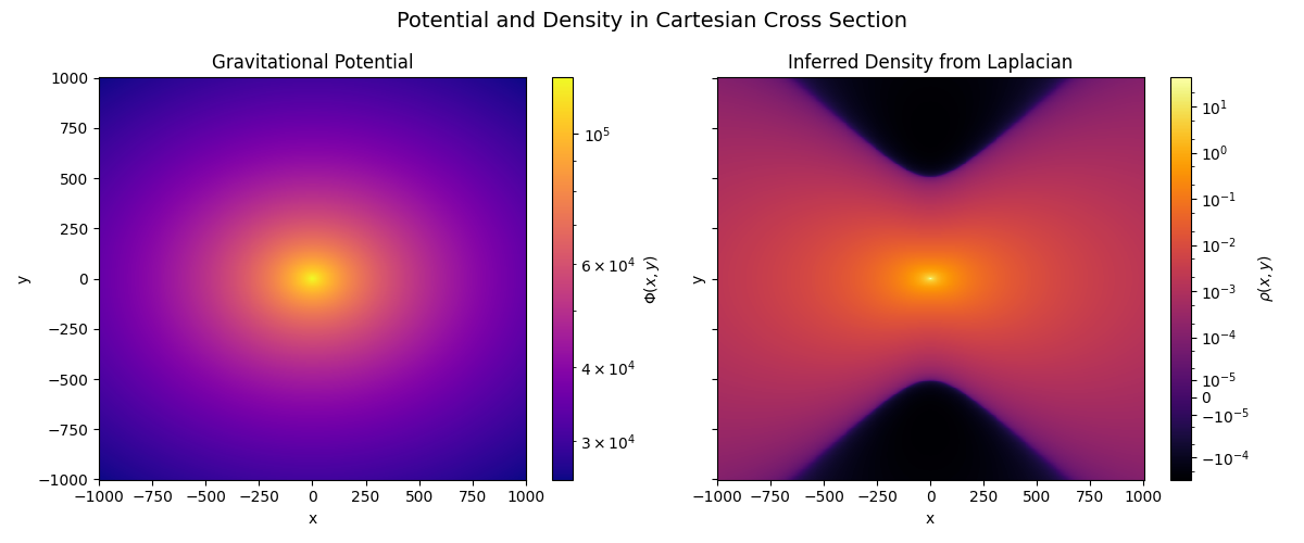
As a final illustration in this example, we can cast this density field to a familiar cartesian grid so that we can visualize the result in 3D. To do so, we’ll use the underlying grid’s construct_domain_interpolator().

# Define Cartesian grid for visualization
# sphinx_gallery_thumbnail_number = 3
x = y = np.linspace(-1000, 1000, 800)
X, Y = np.meshgrid(x, y)

# Interpolators for potential and density fields
potential_interpolator = grid.construct_domain_interpolator(
    field[...], ["xi"], method="cubic", fill_value=None
)
density_interpolator = grid.construct_domain_interpolator(
    density_field[...], ["xi", "theta"], method="cubic", fill_value=None
)

# Convert (X, Y) into oblate coordinates (xi, theta)
XI_GRID, THETA_GRID, _ = grid.coordinate_system.from_cartesian(X, 0, Y)

# Interpolate both fields onto the Cartesian grid
pot_buffer = potential_interpolator(XI_GRID.ravel()).reshape(XI_GRID.shape)
den_buffer = density_interpolator(
    np.stack([XI_GRID.ravel(), THETA_GRID.ravel()], axis=-1)
).reshape(XI_GRID.shape)

# Plot potential and density side-by-side
fig, axes = plt.subplots(1, 2, figsize=(12, 5), sharex=True, sharey=True)

# Gravitational Potential
im0 = axes[0].pcolormesh(X, Y, np.abs(pot_buffer), cmap="plasma", norm=LogNorm())
axes[0].set_title("Gravitational Potential")
axes[0].set_xlabel("x")
axes[0].set_ylabel("y")
cbar0 = plt.colorbar(im0, ax=axes[0], orientation="vertical")
cbar0.set_label(r"$\Phi(x, y)$")

# Density Field
im1 = axes[1].pcolormesh(
    X, Y, den_buffer, norm=AsinhNorm(linear_width=1e-5), cmap="inferno"
)
axes[1].set_title("Inferred Density from Laplacian")
axes[1].set_xlabel("x")
axes[1].set_ylabel("y")
cbar1 = plt.colorbar(im1, ax=axes[1], orientation="vertical")
cbar1.set_label(r"$\rho(x, y)$")

# Finalize layout
plt.suptitle("Potential and Density in Cartesian Cross Section", fontsize=14)
plt.tight_layout()
plt.show()