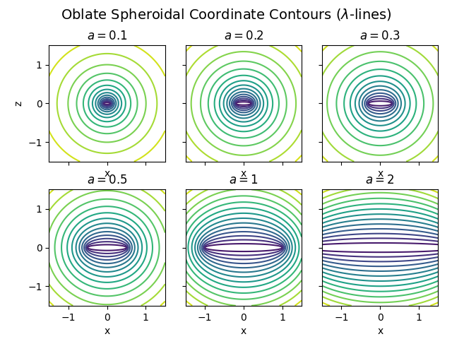
Oblate Spheroidal Coordinates: Effect of Eccentricity

Visualize how the radial coordinate lines (R-contours) in the OblateSpheroidalCoordinateSystem change as a function of eccentricity.

import matplotlib.pyplot as plt

In this example, we’ll showcase a more complex coordinate system: OblateSpheroidalCoordinateSystem.

The oblate spheroidal coordinate system is an orthogonal coordinate system with coordinate variables \((\mu,\nu,\theta)\) for which the \(\mu\) coordinate contours form confocal ellipses.

Hint

The big difference between OblateHomoeoidalCoordinateSystem and OblateSpheroidalCoordinateSystem is that spheroidal coordinates are confocal while homoeoidal coordinates are concentric.

In this example, we’ll show off how to make these coordinate systems and then display some of its properties.

import numpy as np

from pymetric import OblateSpheroidalCoordinateSystem

To visualize, we’ll use an x-z grid and then convert it into the relevant coordinate systems with different eccentricities. We can then plot contours for the effective radius \(\xi\).

# Create the cartesian grid.
x = np.linspace(-1.5, 1.5, 200)
z = np.linspace(-1.5, 1.5, 200)
X, Z = np.meshgrid(x, z)

The class requires an eccentricity parameter when initialized, so we’ll iterate through each of them, create a coordinate system class, and then perform the conversions.

_as = [0.1, 0.2, 0.3, 0.5, 1, 2]

fig, axes = plt.subplots(int(np.ceil(len(_as) / 3)), 3, sharex=True, sharey=True)

for i, a in enumerate(_as):
    ax = axes.ravel()[i]
    csys = OblateSpheroidalCoordinateSystem(a=a)

    # Convert Cartesian (x, z) to native coordinates (λ, μ, φ)
    Lambda, Mu, Phi = csys.from_cartesian(X, 0, Z)

    # Plot λ contours (these correspond to elliptical shells)
    contour = ax.contour(X, Z, Lambda, levels=15, cmap="viridis")
    ax.set_title(f"$a= {a}$")
    ax.set_aspect("equal")
    ax.set_xlabel("x")
    if i == 0:
        ax.set_ylabel("z")

fig.suptitle(r"Oblate Spheroidal Coordinate Contours ($\lambda$-lines)", fontsize=14)
plt.tight_layout()
plt.show()