Note
Go to the end to download the full example code.
Grid Laplacian#
Compute the Laplacian of a field using the grid interface.
import matplotlib.pyplot as plt
import numpy as np
import sympy as sp
In this example, we’ll compute the Laplacian of a field \(\Phi\) in spherical coordinates using
the grids module. For this example, we’ll consider fields of the form
Using the PyMetric interface, we’ll see that this can be done very easily.
Creating the Coordinate System#
The first thing we’ll do is create the coordinate system in PyMetric.
from pymetric import GenericGrid, SphericalCoordinateSystem
from pymetric.differential_geometry import compute_laplacian

coordinate_system = SphericalCoordinateSystem()

# -- Settings for the system -- #
M, K = 10, 3  # These are the parameters for the field.
In PyMetric, coordinate systems can provide symbolic interfaces, which is very helpful here because
it allows us to compute the Laplacian symbolically as well. We’ll use differential_geometry.symbolic
to perform the computation with symbolic expressions from SphericalCoordinateSystem.
# Extract the coordinate symbols
symR, symTheta, symPhi = coordinate_system.axes_symbols
symM, symK = sp.symbols("m k")

# Pull out the metric, Lterm, and metric density
inverse_metric = coordinate_system.inverse_metric_tensor_symbol
Lterm, density = coordinate_system.get_expression(
    "Lterm"
), coordinate_system.get_expression("metric_density")

# Create the field symbolically.
symField = symR**symK * sp.sin(symM * symTheta)

# Determine the Laplacian:
symbolic_laplacian_general = sp.simplify(
    compute_laplacian(
        symField, [symR, symTheta, symPhi], inverse_metric, Lterm, density
    )
)

# Substitute M and K
symbolic_laplacian = sp.simplify(
    symbolic_laplacian_general.subs([(symK, K), (symM, M)])
)
symbolic_laplacian_general
r**(k - 2)*(m*cos(m*theta) + (k*(k - 1) + 2*k - m**2)*sin(m*theta)*tan(theta))/tan(theta)
The result for the general case is a bit tricky!
For the specific case, the result from PyMetric is
2*r*(-44*sin(10*theta) + 5*cos(10*theta)/tan(theta))
For use later, we’ll make this a numerical function too:
true_laplacian = sp.lambdify([symR, symTheta], symbolic_laplacian, "numpy")
Computing the Laplacian Numerically#
We may also perform the computation numerically; which is generally more useful. To do
so, we’ll create a GenericGrid and then use dense_scalar_laplacian().
Creating the Grid#
The first step will be the creation of the grid on which the computations will take place:
# Create the bounding box for the domain.
bbox = [[0, 0, 0], [200, np.pi, 2 * np.pi]]

# Create the coordinates.
# We'll use a small buffer to avoid being on the
# edge of the domain and we'll center the cells.
_buff = 0.1  # The buffer from the edges.
r = np.geomspace(1, 195, 100)
theta, phi = np.linspace(_buff, np.pi - _buff, 100), np.linspace(
    _buff, -_buff + np.pi * 2, 100
)

# Create the grid object.
grid = GenericGrid(coordinate_system, [r, theta, phi], center="cell", bbox=bbox)
Computing the Laplacian#
Now we’re ready to go ahead and compute the Laplacian over the field. All we need to do is build the field and then
we can run the computation.
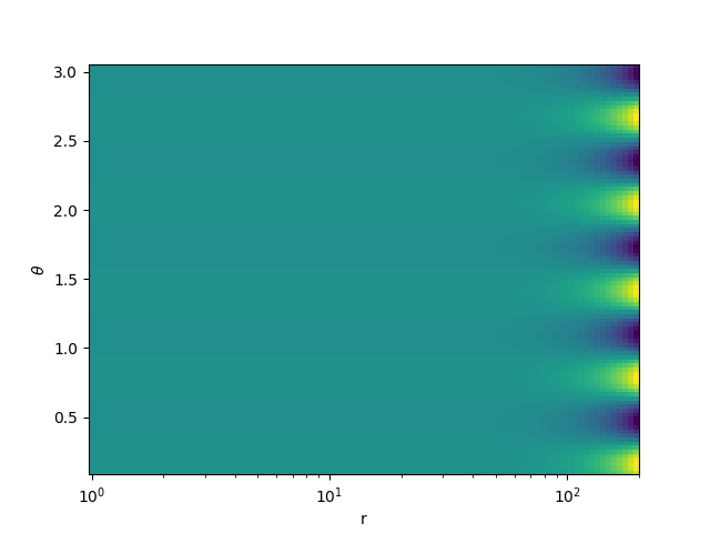
# Create the field function so that we can
# create it on the grid.
field_func = lambda r, theta: r**K * np.sin(M * theta)

# Create the field array. This is a field on
# the r and theta axes.
field_array = grid.compute_function_on_grid(field_func, output_axes=["r", "theta"])

# Create a plot of the field.
fig, axes = plt.subplots(1, 1)

R, THETA = grid.compute_domain_mesh(axes=["r", "theta"])

axes.pcolormesh(R, THETA, field_array)
axes.set_xscale("log")
axes.set_xlabel("r")
axes.set_ylabel(r"$\theta$")
plt.show()
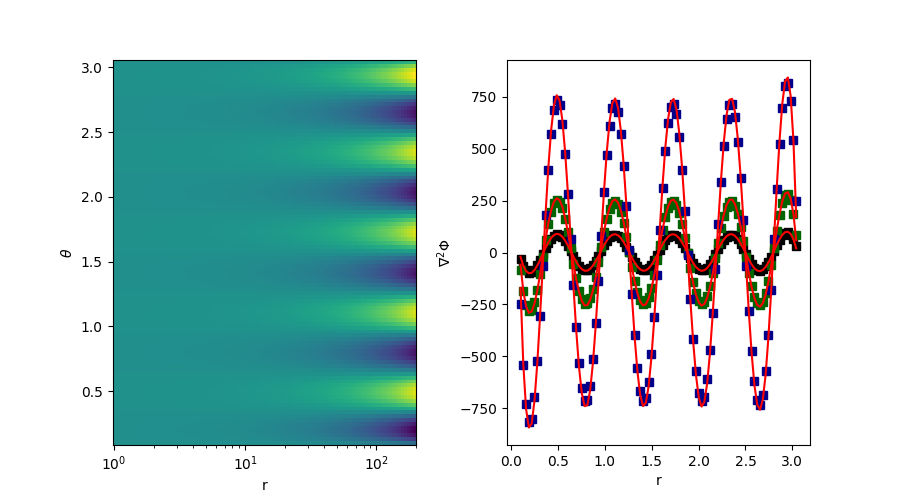
Let’s finally compute the full Laplacian!
# Compute the Laplacian of the field.
field_laplacian = grid.dense_element_wise_laplacian(field_array, ["r", "theta"])

# === Plot === #
# We'll create two plots, one showing the Laplacian,
# and one showing the r=1 cross section of the Laplacian.
fig, axes = plt.subplots(1, 2, figsize=(9, 5), gridspec_kw=dict(wspace=0.3))

# Create the first subplot.
R, THETA = grid.compute_domain_mesh(axes=["r", "theta"])
axes[0].pcolormesh(R, THETA, field_laplacian)
axes[0].set_xscale("log")
axes[0].set_xlabel("r")
axes[0].set_ylabel(r"$\theta$")

# Create the second subplot.
r, theta = grid.compute_domain_coords(axes=["r", "theta"])
axes[1].plot(theta, field_laplacian[0, :], marker="s", color="k", ls="")
axes[1].plot(theta, field_laplacian[20, :], marker="s", color="darkgreen", ls="")
axes[1].plot(theta, field_laplacian[40, :], marker="s", color="darkblue", ls="")

axes[1].plot(theta, true_laplacian(r[20], theta), color="red")
axes[1].plot(theta, true_laplacian(r[0], theta), color="red")
axes[1].plot(theta, true_laplacian(r[40], theta), color="red")

axes[1].set_xlabel("r")
axes[1].set_ylabel(r"$\nabla^2 \Phi$")
plt.show()
Total running time of the script: (0 minutes 0.889 seconds)