Fields: Overview#
In Pymetric, fields (fields) are the most important data structure for representing
numerical quantities defined over geometric grids. They provide a uniform interface
for scalar, vector, and tensor-valued data in arbitrary coordinate systems.
Operationally, fields behave similarly to NumPy arrays. They support arithmetic, slicing, unit-aware computation (via unyt), and broadcasting— but with full awareness of the spatial domain and coordinate system they inhabit.
This document provides an introductory look at these objects and some of the things you can do with them!
What is a Field?#
Fields are high-level objects in PyMetric which hold structured data on a specific
geometric grid (see grids and Geometric Grids: General Info), which in turn contains an underlying
coordinate system (see coordinates and Coordinate Systems: General Info). They abstract away the complexity
of differential geometry and provide:
Grid-aligned storage and shape metadata
Physical units (if present) and element-wise structure (e.g., tensors)
Support for arithmetic, reduction, reshaping, and numerical operations
Integration with symbolic and numerical differential operators
Each field consists of one or more components (FieldComponent), and each component stores
its data in a buffer (BufferBase). The field manages how those components are laid out
and ensures consistency with the grid.
Sparse Fields vs. Dense Fields#
Pymetric currently supports two major field representations:
Dense Fields (
DenseFieldand descendants):Are composed of a single component of a specific shape. For example, in spherical coordinate system (3D), a vector field would be densely represented with a single component of shape
(..., 3).For tensor fields specifically, dense representations are required to have all of the necessary indices, even if they are zero. Thus, dense fields are often simpler to work with and have more efficient numerical operations; however, in cases where only some components are relevant, a large memory and computation overhead is incurred to handle data that isn’t necessary.
Sparse Fields (
SparseFieldand descendants)(planned):Are composed of multiple components all of which are scalar components on the grid. Thus, for a vector field in spherical coordinates, there would be 3 separate components in a sparse representation, one for each direction.
For tensor fields, the great advantage of sparse representation is that missing components can be treated as implicitly zero. Thus, a vector field with only a \(\hat{\bf r}\) component would only need one scalar component.
Important
Support for sparse operations is planned but not yet implemented.
Buffers and Components#
Each field consists of one or more components (FieldComponent), and each component stores
its data in a buffer (BufferBase). Here’s how they relate:
Buffers are the raw data containers. They abstract over memory/storage backends (e.g., NumPy arrays, unyt arrays with units, or HDF5-backed arrays). Buffers provide arithmetic, indexing, and I/O functionality.
FieldComponents wrap a buffer and associate it with a subset of the grid axes and an element shape. This allows them to represent scalar values, vectors, or tensors.
Fields manage one or more components and provide the full user interface.
This design separates memory layout (buffers), spatial semantics (components), and user interaction (fields), enabling modularity and extensibility.
For the most part, users won’t have need to interact with buffers at all and with components only rarely. They are largely just logical separators for code maintainability. Nonetheless, some operations do expose lower level backends and it is useful to understand the classes involved when such instances arise.
Special Types of Fields#
There are two “parent field classes”: SparseField and DenseField. In turn,
various special field types descent from these two archetypes. The most important of these are tensor fields,
which provide marginally more structure to their base classes while allowing for fully covariant computations like
divergences, curls, etc. These are stored in the fields.tensors module.
For most scientific workflows, users should use the DenseTensorField class which provides
all of the relevant structure for things like vectors, co-vectors, scalar fields, etc.
Creating Fields#
There are a number of ways to create fields in PyMetric, largely depending on what information the user wishes to provide in creating the instance. In this section, we’ll walk through some of the various options that are most common.
Building a Field from Components#
Perhaps the most direct way to construct a field is to first create one or more instances of
FieldComponent. This is especially true when using the default
constructor—i.e., calling DenseField(...)—which expects the data to already be wrapped
in a fully-formed FieldComponent. The constructor does not accept raw arrays,
functions, or other input types directly. For those use cases, convenience constructors should be used instead (see below).
To construct a dense field (DenseField) directly, the user must provide
a grid (see grids) and a single component:
from pymetric import DenseField, CartesianCoordinateSystem2D, GenericGrid, FieldComponent

cs = CartesianCoordinateSystem2D()
x, y = [0, 1, 2], [0, 1, 2]
g = GenericGrid(cs, [x, y])
component = FieldComponent.zeros(g,['x','y'])
f = DenseField(g,component)
To construct a dense tensor field (DenseTensorField) directly, the user must provide
a grid (see grids), a single component, and (optionally) the signature of the tensor. For example,
a scalar field can be created with
from pymetric import DenseField, CartesianCoordinateSystem2D, GenericGrid, FieldComponent

cs = CartesianCoordinateSystem2D()
x, y = [0, 1, 2], [0, 1, 2]
g = GenericGrid(cs, [x, y])
component = FieldComponent.zeros(g,['x','y'])
f = DenseField(g,component)
Warning
A valid tensor field component must have an element shape like (Ndim, Ndim, ...) or
an error is raised. This is reflective of the dense representation convention where all indices
are required.
A vector field looks like
from pymetric import DenseField, CartesianCoordinateSystem2D, GenericGrid, FieldComponent

cs = CartesianCoordinateSystem2D()
x, y = [0, 1, 2], [0, 1, 2]
g = GenericGrid(cs, [x, y])
component = FieldComponent.zeros(g,['x','y'],element_shape=(2,))
f = DenseField(g,component)
To create a covector field, signature should be specified:
from pymetric import DenseField, CartesianCoordinateSystem2D, GenericGrid, FieldComponent

cs = CartesianCoordinateSystem2D()
x, y = [0, 1, 2], [0, 1, 2]
g = GenericGrid(cs, [x, y])
component = FieldComponent.zeros(g,['x','y'],element_shape=(2,))
f = DenseField(g,component,signature=(-1,))
Important
Not yet implemented.
Building a Generic Field#
Like most array-manipulation libraries, PyMetric provides a number of field entry points for building
empty fields as well as fields filled with either 0 or 1. These mirror the standard behavior of functions
like numpy.zeros(), numpy.ones(), etc.
Many classes in PyMetric implement these as methods (i.e. BufferBase, GridBase,
and FieldComponent), including all of the field classes. The call signatures vary somewhat
between methods to account for differences in structure:
For dense fields, the operations works just like one would expect.
from pymetric import DenseField, CartesianCoordinateSystem2D, GenericGrid, FieldComponent

cs = CartesianCoordinateSystem2D()
x, y = [0, 1, 2], [0, 1, 2]
g = GenericGrid(cs, [x, y])
component = FieldComponent.zeros(g,['x','y'])
f = DenseField.zeros(g, ['x']) # Create scalar field over x axis of g.
A number of options are available to determine how the underlying buffer behaves, what
shape the field has, etc. For details, look at zeros().
For tensor fields, the operations works a little bit different than for DenseField.
Instead of controlling the shape of the field with the element_shape= kwarg, zeros()
takes 1 additional positional argument: rank (the rank of the tensor) and uses that to determine the
correct (dense) shape. Additionally, signature= may be used to specify the variance.
from pymetric import DenseTensorField, CartesianCoordinateSystem2D, GenericGrid, FieldComponent

cs = CartesianCoordinateSystem2D()
x, y = [0, 1, 2], [0, 1, 2]
g = GenericGrid(cs, [x, y])
component = FieldComponent.zeros(g,['x','y'])
f = DenseTensorField.zeros(g, ['x'], 2) # Create rank 2 field over x axis of g.

# For a covector, you might need:
f = DenseTensorField.zeros(g, ['x'], 1, signature=(-1,))
A number of options are available to determine how the underlying buffer behaves, what
shape the field has, etc. For details, look at zeros().
Important
Not yet implemented.
In addition to the standard ones(), zeros(), and
full(), all dense field representations also implement a from_array()
method to allow users to provide a generic buffer as the basis for a new field.
Advanced Construction Methods#
In addition to the core construction methods presented above, a few additional methods are available to construct fields
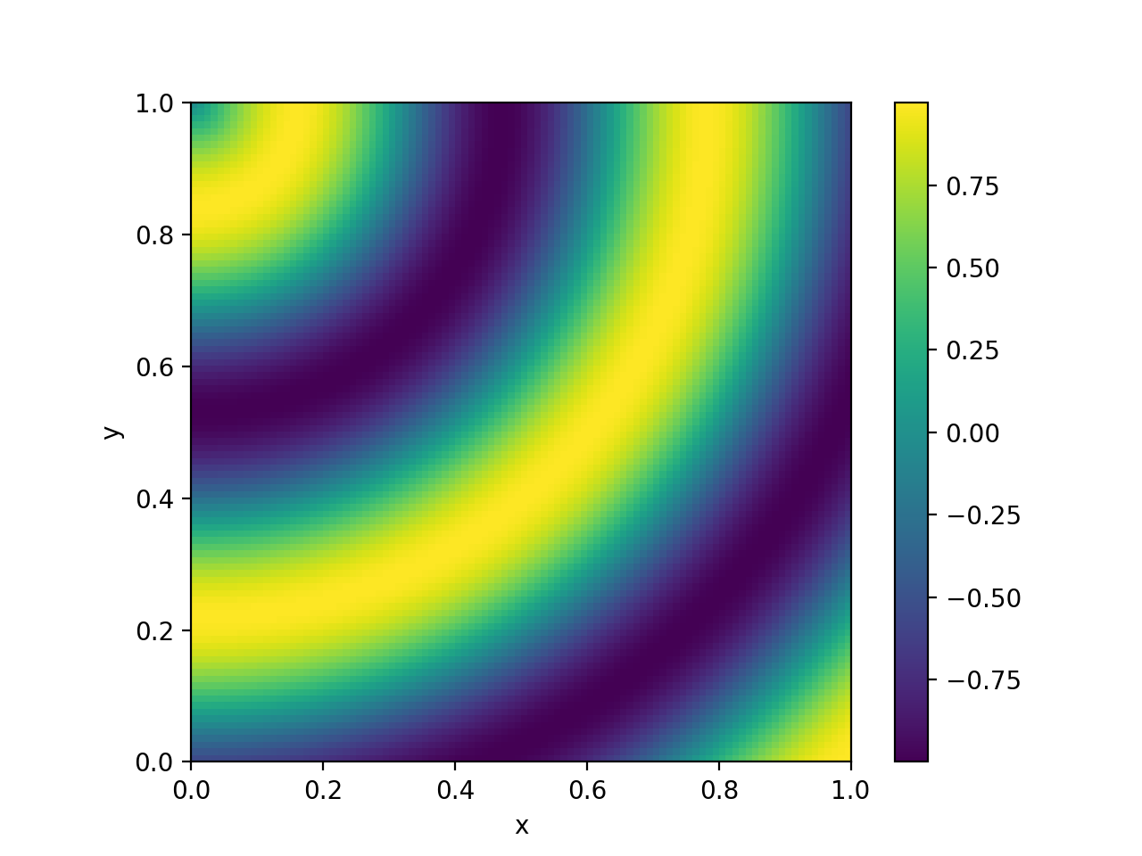
from more esoteric origins. The most significant of these is the from_function() which allows
users to create fields by specifying directly a function \(f(x^1,x^2,\ldots,x^n)\). The following example illustrates
the basic usage:
import numpy as np
from pymetric import DenseField, CartesianCoordinateSystem2D, GenericGrid
import matplotlib.pyplot as plt

# Create the coordinate system and the grid.
cs = CartesianCoordinateSystem2D()
x, y = (np.linspace(0,1,100),
        np.linspace(0,1,100))
g = GenericGrid(cs, [x, y])

# Define a function of the coords.
func = lambda _x,_y: np.sin(10*np.sqrt(_x**2+_y**2))

# Create the dense field from the function.
f = DenseField.from_function(func, g, ['x','y'])

fig,axes = plt.subplots(1,1)
Q = axes.imshow(f[...].T,extent=(0,1,0,1))
axes.set_xlabel('x')
axes.set_ylabel('y')
plt.colorbar(Q,ax=axes)
plt.show()
(Source code, png, hires.png, pdf)
Field Properties and Data Access#
Once fields are created, they offer a rich interface for interacting with both their geometric context and numerical data. This section explains the core capabilities fields provide for data access, metadata retrieval, and computational manipulation.
Properties of Fields#
Fields are built on top of structured grids and are deeply aware of their spatial and element-wise structure. Every field, whether sparse or dense, encodes both where data lives (i.e., the grid and its axes) and what kind of data it holds (e.g., scalars, vectors, tensors).
Linkage to grid, axes (dense), and coordinate system.
element_shape, spatial_shape,element_ndim, spatial_ndim, etc.
Point readers to the API documentation for more details.
Some key properties include:
grid: The underlyingGridBaseinstance that the field lives on. This contains coordinate information, dimensions, and domain metadata.axes: A list of the axes over which the field spans.spatial_shape: The shape of the field over its spatial axes.element_shape: The trailing shape of the data, representing its tensor structure .units: If unit-aware buffers (e.g., via unyt) are used, this indicates the physical units attached to the field.
Accessing Field Data#
A major difference between sparse and dense field representations is the syntax for data access. The tabs below summarize how data access behaves in each case:
Dense fields behave very much like regular NumPy arrays. Indexing directly into a field returns the corresponding data slice from the single component buffer. This means you can treat dense fields as array-like objects for most numerical and visualization operations:
val = field[i, j]           # Scalar or element value at grid index (i, j)
slice = field[::2, ::2]     # Subsampled field
comp = field[..., 1]        # Slice of a vector/tensor component
All operations are performed on the raw buffer data (NumPy, unyt, or HDF5), and indexing reflects that behavior. If the field has a unit-aware backend (e.g., unyt_array), the result will preserve units.
You can explicitly retrieve representations using:
as_array(): returns a NumPy array (units stripped).as_unyt_array(): returns a unyt_array with units.as_buffer_core(): returns the native backend array (e.g., h5py.Dataset).as_buffer_repr(): returns a NumPy-compatible representation for ufuncs.
These methods are particularly useful when exporting to disk, performing raw NumPy operations, or applying custom logic where backend control is needed.
Sparse fields (planned) contain multiple components, each aligned with a subset of axes and representing a scalar value.
Accessing the field returns an individual FieldComponent, which must then be indexed:
component = field[0]        # Return the first component
value = component[i, j]       # Access value at spatial index
Sparse fields are useful when only a few components of a tensor are needed or when symbolic sparsity is important (e.g., fields with known zeros). While dense fields always store all components (even if zero), sparse fields can reduce memory and computation by omitting unnecessary entries.
Note: Because sparse field support is not yet implemented, the behavior outlined above is aspirational and may change.
Hint
When accessing fields in user constructed pipelines, it is often useful to be conscious of how access patterns impact memory usage; particularly for buffers which have lazy-loading behaviors.
Broadcasting and Iteration#
Talk about the ability to broadcast to arrays and other buffer types in new axes and also as general base types.
Talk about broadcasting to new axes and reducing to new axes.
In addition, a couple other access patterns:
Iterating through chunks of the data;
casting to axes (Dense -> sparse can do the same with each component separately)
cutting to axes (Dense -> sparse can do the same with each component seperately.)
Field iterpolation.