grids.mixins.mathops.DenseMathOpsMixin.dense_vector_divergence_contravariant#
- DenseMathOpsMixin.dense_vector_divergence_contravariant(vector_field: _Buffer | _SupportsArray[dtype[Any]] | _NestedSequence[_SupportsArray[dtype[Any]]] | complex | bytes | str | _NestedSequence[complex | bytes | str], field_axes: Sequence[str], /, out: _Buffer | _SupportsArray[dtype[Any]] | _NestedSequence[_SupportsArray[dtype[Any]]] | complex | bytes | str | _NestedSequence[complex | bytes | str] | None = None, Dterm_field: _Buffer | _SupportsArray[dtype[Any]] | _NestedSequence[_SupportsArray[dtype[Any]]] | complex | bytes | str | _NestedSequence[complex | bytes | str] | None = None, derivative_field: _Buffer | _SupportsArray[dtype[Any]] | _NestedSequence[_SupportsArray[dtype[Any]]] | complex | bytes | str | _NestedSequence[complex | bytes | str] | None = None, *, in_chunks: bool = False, edge_order: Literal[1, 2] = 2, output_axes: Sequence[str] | None = None, pbar: bool = True, pbar_kwargs: dict | None = None, **kwargs)[source]#
Compute the divergence of a contravariant vector field on a grid.
For a contravariant vector field \(V^\mu\), the divergence is given by:
\[\nabla \cdot V = \frac{1}{\rho} \partial_\mu(\rho V^\mu) = \partial_\mu V^\mu + V^\mu \frac{\partial_\mu \rho}{\rho}\]This expanded form is used for improved numerical stability and implemented as a sum of a standard derivative and a geometry-aware “D-term”.
- Parameters:
vector_field (
array-like) – The vector field on which to compute the divergence. This should be an array-like object with a compliant shape (see Notes below).field_axes (
listofstr) – The coordinate axes over which the field spans. This should be a sequence of strings referring to the various coordinates of the underlyingcoordinate_systemof the grid. For each element in field_axes, field’s i-th index should match the shape of the grid for that coordinate. (See Notes for more details).out (
array-like, optional) – An optional buffer in which to store the result. This can be used to reduce memory usage when performing computations. The shape of out must be compliant with broadcasting rules (see Notes). out may be a buffer or any other array-like object.Dterm_field (
array-like, optional) – The D-term field for the specific coordinate system. This can be specified to improve computation speed; however, it can also be derived directly from the grid’s coordinate system. If it is provided, it should be compliant with the shaping / broadcasting rules (see Notes).derivative_field (
array-like, optional) – The first derivatives of the vector_field. derivative_field can be specified to improve computational speed or to improve accuracy if the derivatives are known analytically; however, they can also be computed numerically if not provided. If derivative_field is provided, it must comply with the shaping / broadcasting rules (see Notes).output_axes (
listofstr, optional) –The axes of the coordinate system over which the result should span. By default, output_axes is the same as field_axes and the output field matches the span of the input field.
This argument may be specified to expand the number of axes onto which the output field is computed. output_axes must be a superset of the field_axes.
in_chunks (
bool, optional) – Whether to perform the computation in chunks. This can help reduce memory usage during the operation but will increase runtime due to increased computational load. If input buffers are all fully-loaded into memory, chunked performance will only marginally improve; however, if buffers are lazy loaded, then chunked operations will significantly improve efficiency. Defaults toFalse.edge_order (
{1, 2}, optional) – Order of the finite difference scheme to use when computing derivatives. Seenumpy.gradient()for more details on this argument. Defaults to2.pbar (
bool, optional) – Whether to display a progress bar when in_chunks=True.pbar_kwargs (
dict, optional) – Additional keyword arguments passed to the progress bar utility. These can be any valid arguments totqdm.tqdm().**kwargs – Additional keyword arguments passed to
dense_vector_divergence_contravariant().
- Returns:
The computed partial derivatives. The resulting array will have a field shape matching the grid’s shape over the output_axes and an element shape matching that of field but with an additional (ndim,) sized dimension containing each of the partial derivatives for each index.
- Return type:
array-like
Notes
Broadcasting and Array Shapes:
The input
vector_fieldmust have a very precise shape to be valid for this operation. If the underlying grid (including ghost zones) has shapegrid_shape = (G_1,...,G_ndim), then the spatial dimensions of the field must match exactlygrid_shape[axes].vector_fieldshould have 1 additional dimension representing the vector components which must have a size ofndim. The resulting output array will be a scalar field over the relevant grid axes.Thus, if a
(G1,G3,ndim)field is passed withfield_axes = ['x','z'](in cartesian coordinates), then the resulting output array will have shape(G1,G3).If
output_axesis specified, then that resulting grid will be broadcast to any additional grid axes necessary.If either
derivative_fieldorDterm_fieldare not provided, then they must each be provided over theoutput_axes(if they are specified, otherwisefield_axes). TheDterm_fieldshould have 1 additional dimension of sizendimcontaining each of the elements of the covector field. Thederivative_fieldmust also be specified over theoutput_axes(if they are specified, otherwisefield_axes), but can have any number of elements in its 1 additional dimension (corresponding to the set of non-zero derivatives).When
outis specified, it must match (exactly) the expected output buffer shape or an error will arise.Chunking Semantics:
When
in_chunks=True, chunking is enabled for this operation. In that case, theoutbuffer is filled iteratively by performing computations on each chunk of the grid over the specified output_axes. When the computation is performed, each chunk is extracted with an additional 1-cell halo to ensure thatnumpy.gradient()attains its maximal accuracy on each chunk.Note
Chunking is (generally) only useful when
outandvector_fieldare array-like lazy-loaded buffers like HDF5 datasets. In those cases, the maximum memory load is only that required to load each individual chunk. If theoutbuffer is not specified, it is allocated fully anyways, making chunking somewhat redundant.Examples
In Spherical Coordinates, the divergence is
\[\nabla \cdot V = \frac{1}{r^2}\partial_r\left(r^2V^r\right) + \frac{1}{\sin \theta} \partial_\theta \left(\sin \theta V^\theta\right) + \partial_\phi V^\phi.\]As such, if \(V^\mu = \left(r cos \theta,\; \sin\theta,\; 0\right)\), then
\[\nabla \cdot V = \frac{\cos \theta}{r^2}\partial_r r^3 + \frac{1}{\sin \theta}\partial_\theta \sin^2\theta = 5 \cos \theta.\]To see this numerically, we can do the following:
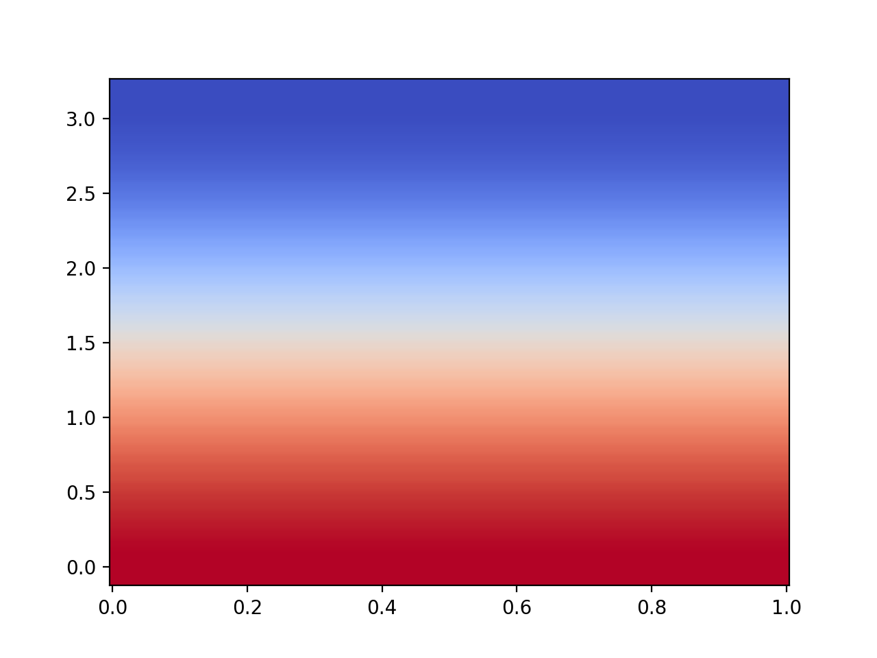
>>> from pymetric.grids.core import UniformGrid
>>> from pymetric.coordinates import SphericalCoordinateSystem
>>> import matplotlib.pyplot as plt
>>>
>>> # Create the coordinate system
>>> cs = SphericalCoordinateSystem()
>>>
>>> # Create the grid
>>> grid = UniformGrid(cs,[[0,0,0],[1,np.pi,2*np.pi]],
...                   [500,50,50],
...                   chunk_size=[50,50,50],
...                   ghost_zones=[2,2,2],center='cell')
>>>
>>> # Create the field
>>> R, THETA = grid.compute_domain_mesh(origin='global',axes=['r','theta'])
>>> Z = np.stack([R * np.cos(THETA), np.sin(THETA), np.zeros_like(R)],axis=-1)
>>> Z.shape
(504, 54, 3)
>>>
>>> # Compute the divergence.
>>> DivZ = grid.dense_vector_divergence_contravariant(Z,['r','theta'],in_chunks=True)
>>>
>>> fig,axes = plt.subplots(1,1)
>>> _ = axes.imshow(DivZ.T,aspect='auto',origin='lower',extent=grid.gbbox.T.ravel(),vmin=-5,vmax=5,cmap='coolwarm')
>>> plt.show()
(
Source code,png,hires.png,pdf)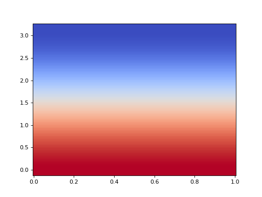