pisces.math_utils.random_fields.generate_zh11_power_spectrum

pisces.math_utils.random_fields.generate_zh11_power_spectrum(amplitude: float = 1.0, k0: float = 1.0, k1: float = 5.0) → Callable

Generate a Kolmogorov-like power spectrum following ZuHone et al. (2011).

The spectrum is defined as

\[P(k) = A \, k^{-11/3} \, \exp\!\left[-\left(\frac{k}{k_0}\right)^2\right] \exp\!\left[-\frac{k_1}{k}\right],\]

where

• \(A\) is the normalization amplitude,

• \(k_0\) sets the high-wavenumber (small-scale) cutoff,

• \(k_1\) sets the low-wavenumber (large-scale) cutoff.

Parameters:

• amplitude (float, optional) – Normalization amplitude \(A\). Default is 1.0.

• k0 (float, optional) – High-wavenumber cutoff \(k_0\). Default is 1.0.

• k1 (float, optional) – Low-wavenumber cutoff \(k_1\). Default is 5.0.

Returns:

A function P(kx, ky, ...) that takes arrays of wavenumber components and returns the ZuHone+11 spectrum evaluated on that grid.

Return type:

Callable

Examples

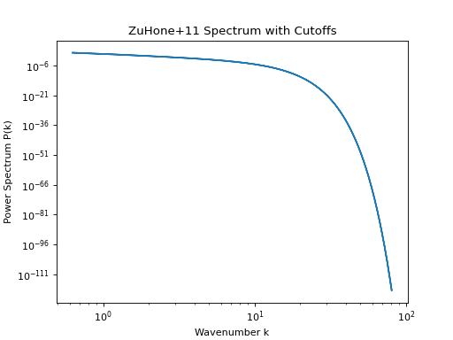
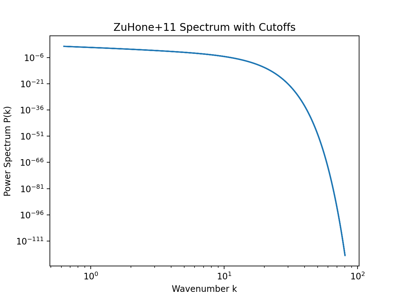
from pisces.math_utils.random_fields import generate_zh11_power_spectrum
L, n = 10.0, 256
k_grid = np.fft.fftfreq(n, d=L/n) * 2 * np.pi
k_mag = np.abs(k_grid)
ps_func = generate_zh11_power_spectrum(amplitude=1.0, k0=5.0, k1=0.5)
ps_array = ps_func(k_mag)

import matplotlib.pyplot as plt
plt.loglog(k_mag[1:], ps_array[1:])  # skip k=0
plt.xlabel('Wavenumber k')
plt.ylabel('Power Spectrum P(k)')
plt.title('ZuHone+11 Spectrum with Cutoffs')
plt.show()

(Source code, png, hires.png, pdf)