
pisces.math_utils.random_fields.generate_power_law_power_spectrum#
- pisces.math_utils.random_fields.generate_power_law_power_spectrum(amplitude: float = 1.0, k0: float = 1.0, slope: float = -3.6666666666666665) Callable[source]#
Generate a power-law power spectrum function.
A power-law spectrum is defined by
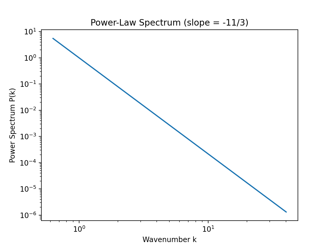
\[P(k) = A \left( \frac{k}{k_0} \right)^{\alpha},\]where \(A\) is the amplitude, \(k_0\) is a reference wavenumber for normalization, and \(\alpha\) is the slope. A slope of \(\alpha = -11/3\) corresponds to the Kolmogorov scaling for incompressible turbulence.
- Parameters:
- Returns:
A function
P(kx, ky, ...)that takes arrays of wavenumber components and returns the power-law spectrum evaluated on that grid.- Return type:
Callable
Examples
from pisces.math_utils.random_fields import generate_power_law_power_spectrum
L, n = 10.0, 128
k_grid = np.fft.fftfreq(n, d=L/n) * 2 * np.pi
k_mag = np.abs(k_grid)
power_spectrum = generate_power_law_power_spectrum(slope=-11/3)
ps_array = power_spectrum(k_mag)

import matplotlib.pyplot as plt
plt.loglog(k_mag[1:], ps_array[1:])  # skip k=0
plt.xlabel('Wavenumber k')
plt.ylabel('Power Spectrum P(k)')
plt.title('Power-Law Spectrum (slope = -11/3)')
plt.show()
(
Source code,png,hires.png,pdf)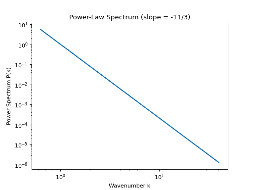