
pisces.math_utils.random_fields.generate_gaussian_cutoff_power_spectrum#
- pisces.math_utils.random_fields.generate_gaussian_cutoff_power_spectrum(amplitude: float = 1.0, k0: float = 1.0, sigma: float = 1.0) Callable[source]#
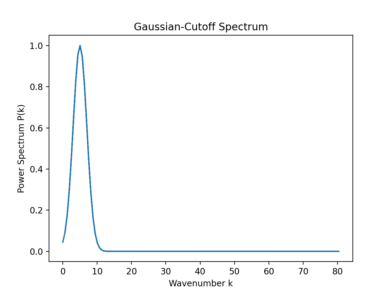
Generate a Gaussian-cutoff power spectrum function.
The Gaussian-cutoff spectrum is defined by
\[P(k) = A \exp\!\left[-\frac{1}{2} \left(\frac{k - k_0}{\sigma}\right)^2\right],\]where \(A\) is the amplitude, \(k_0\) is the central wavenumber, and \(\sigma\) controls the width of the Gaussian. This spectrum is peaked around \(k_0\) and falls off rapidly away from the peak.
- Parameters:
- Returns:
A function
P(kx, ky, ...)that takes arrays of wavenumber components and returns the Gaussian-cutoff spectrum.- Return type:
Callable
Examples
from pisces.math_utils.random_fields import generate_gaussian_cutoff_power_spectrum
L, n = 10.0, 256
k_grid = np.fft.fftfreq(n, d=L/n) * 2 * np.pi
k_mag = np.abs(k_grid)
power_spectrum = generate_gaussian_cutoff_power_spectrum(k0=5.0, sigma=2.0)
ps_array = power_spectrum(k_mag)

import matplotlib.pyplot as plt
plt.plot(k_mag, ps_array)
plt.xlabel('Wavenumber k')
plt.ylabel('Power Spectrum P(k)')
plt.title('Gaussian-Cutoff Spectrum')
plt.show()
(
Source code,png,hires.png,pdf)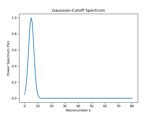