pisces.math_utils.random_fields.generate_kolmogorov_power_spectrum

pisces.math_utils.random_fields.generate_kolmogorov_power_spectrum(amplitude: float = 1.0, k0: float = 1.0, k_cut: float | None = None) → Callable

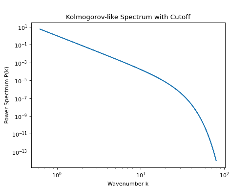
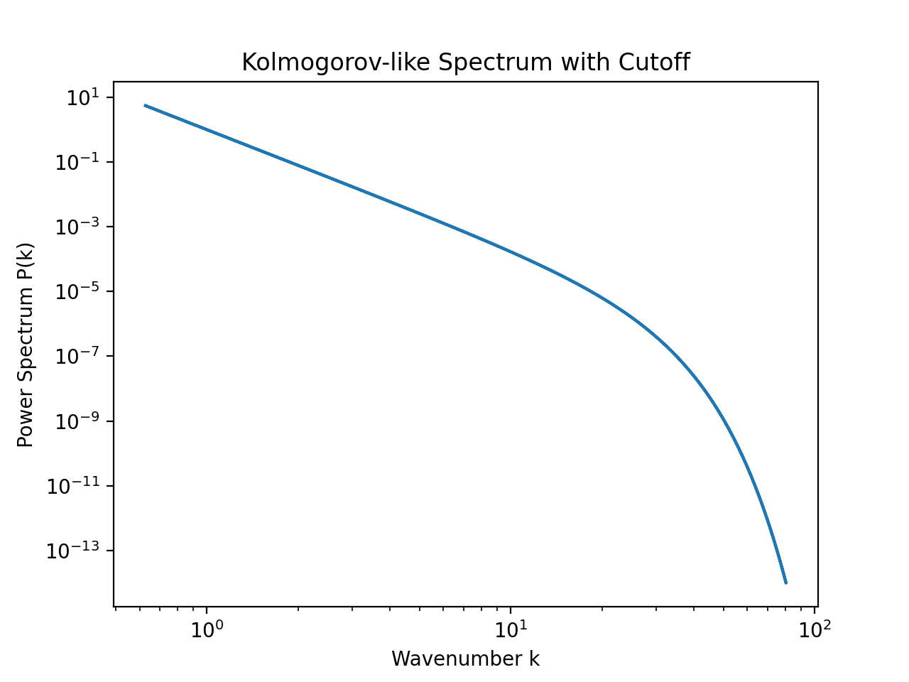
Generate a Kolmogorov-like turbulence power spectrum function.

The Kolmogorov turbulence scaling predicts an energy spectrum \(E(k) \propto k^{-5/3}\), which corresponds to a power spectrum \(P(k) \propto k^{-11/3}\) in three dimensions. This function implements

\[P(k) = A \left(\frac{k}{k_0}\right)^{-11/3} \exp\!\left[-\left(\frac{k}{k_\mathrm{cut}}\right)^2\right],\]

where the exponential cutoff is optional and only applied if \(k_\mathrm{cut}\) is specified.

Parameters:

• amplitude (float, optional) – Normalization amplitude \(A\). Default is 1.0.

• k0 (float, optional) – Reference wavenumber \(k_0\). Default is 1.0.

• k_cut (float, optional) – High-wavenumber cutoff \(k_\mathrm{cut}\). If provided, applies a Gaussian suppression factor. Default is None.

Returns:

A function P(kx, ky, ...) that takes arrays of wavenumber components and returns the Kolmogorov-like spectrum.

Return type:

Callable

Examples

from pisces.math_utils.random_fields import generate_kolmogorov_power_spectrum
L, n = 10.0, 256
k_grid = np.fft.fftfreq(n, d=L/n) * 2 * np.pi
k_mag = np.abs(k_grid)
power_spectrum = generate_kolmogorov_power_spectrum(amplitude=1.0, k0=1.0, k_cut=20.0)
ps_array = power_spectrum(k_mag)

import matplotlib.pyplot as plt
plt.loglog(k_mag[1:], ps_array[1:])  # skip k=0
plt.xlabel('Wavenumber k')
plt.ylabel('Power Spectrum P(k)')
plt.title('Kolmogorov-like Spectrum with Cutoff')
plt.show()

(Source code, png, hires.png, pdf)