Derived and Computed Gravitational Potentials

See how profiles can provide both numeric and analytical derived quantities.

In this example, we’ll take the NFW profile (NFWDensityProfile) and the Einasto profile (EinastoDensityProfile) and compare their gravitational potentials. Because the NFW profile has an analytic expression for its potential, it is included in the class as a derived quantity. The Einasto profile does not have an analytic expression, so we will compute it numerically using the general-purpose method. In doing both, we will see how to access both derived and computed quantities from profiles.

Hint

You can read more about derived and computed quantities in the profiles_overview.

Setup

To get started, we’ll import the necessary libraries and define our profile parameters and construct the resulting profile objects.

import matplotlib.pyplot as plt

# Imports
import numpy as np
import unyt

from pisces.profiles.density import EinastoDensityProfile, NFWDensityProfile

# Constants and parameters
rho_0 = unyt.unyt_quantity(1.0, "Msun/kpc**3")
r_s = unyt.unyt_quantity(10.0, "kpc")

# Instantiate profiles
nfw = NFWDensityProfile(rho_0=rho_0, r_s=r_s)
einasto = EinastoDensityProfile(rho_0=rho_0, r_s=r_s, alpha=0.9)

Derived Profiles

As described in the documentation, profiles can carry with them analytically derived quantities such as their gravitational potential, circular velocity, and mass profiles. These are accessible via the get_derived_profile() method. You can also see a list of the available derived profiles via the list_derived_profiles.

# Look at which derived profiles are available
print("NFW derived profiles:", nfw.list_derived_profiles())
print("Einasto derived profiles:", einasto.list_derived_profiles())

NFW derived profiles: ['derivative', 'enclosed_mass', 'gravitational_potential', 'gravitational_field']
Einasto derived profiles: ['derivative']

As you can see, the NFW profile has a derived gravitational potential, while the Einasto profile does not. This is because the NFW potential has an analytic expression, while the Einasto potential does not.

Nonetheless, we can still compute the Einasto potential numerically using the general-purpose method compute_gravitational_potential().

# Start with the NFW profile and it's derived gravitational potential
nfw_potential = nfw.get_derived_profile("gravitational_potential")

# Now the Einasto profile and its computed gravitational potential
r = unyt.unyt_array(np.logspace(-1, 2, 300), "kpc")  # 0.1–100 kpc
einasto_potential = einasto.compute_gravitational_potential(r, units="km**2/s**2")

# We'll also do NFW computationally to ensure fidelity.
nfw_potential_computed = nfw.compute_gravitational_potential(r, units="km**2/s**2")

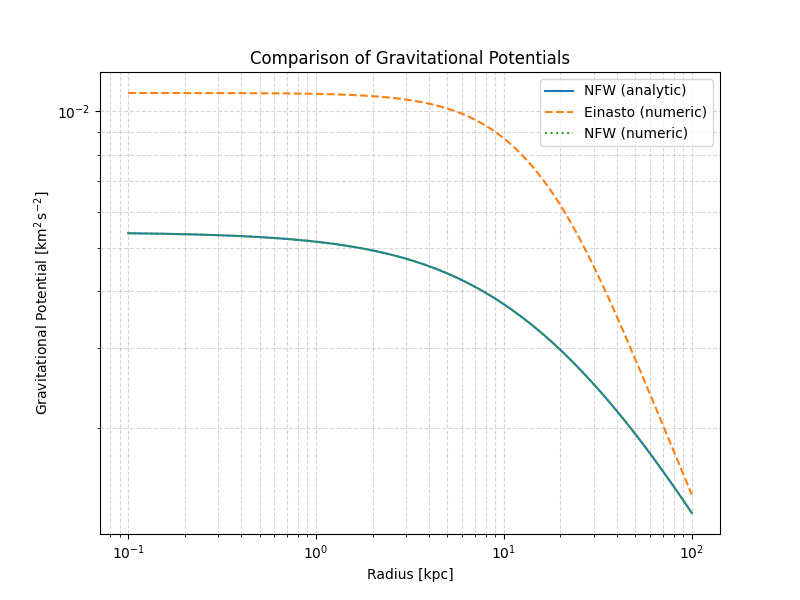
Plot Comparison

For the NFW profile, we evaluate its derived gravitational potential at the same radii.

phi_nfw = nfw_potential(r).to("km**2/s**2")
phi_einasto = einasto_potential  # already computed above

plt.figure(figsize=(8, 6))
plt.loglog(r.to("kpc"), -phi_nfw, label="NFW (analytic)")
plt.loglog(r.to("kpc"), -phi_einasto, label="Einasto (numeric)", ls="--")
plt.loglog(r.to("kpc"), -nfw_potential_computed, label="NFW (numeric)", ls=":")

plt.xlabel("Radius [kpc]")
plt.ylabel(r"Gravitational Potential [$\mathrm{km^2 \, s^{-2}}$]")
plt.title("Comparison of Gravitational Potentials")
plt.legend()
plt.grid(True, which="both", ls="--", alpha=0.5)
plt.show()